Awesome User Activation
27 March, 2018
In a previous analysis we used some simple EDA techniques to explore “activation” for new Buffer users. In another analysis we explored possible activation metrics for Business customers.
In this analysis we’ll use a similar approaches to explore what activation could look like for Awesome customers. We’ll define success in this case as being retained – not cancelling the subscription – for at least 12 months.
The features we’ll analyze are:
- The number of days that the user was a Buffer user before starting the subscription.
- Whether or not the subscription had an associated trial.
- The number of profiles the user had 28 days after the subscription started.
- The number of distinct days in which updates were created during the first four weeks on the plan.
- The number of distinct weeks in which updates were created during the first four weeks on the plan.
- The number of updates per profile created during the four weeks on the plan.
Let’s collect the data.
Data Collection
We’ll run the query below to collect the data we need. We only want to get Awesome customers that have paid us successfully and that were active at least 12 months ago. We don’t know if Awesome subscriptions that were started in the past year will be retained for 12 months or not.
with awesome_users as (
  select
    s.id as subscription_id
    , s.customer as customer_id
    , u.id as user_id
    , date(u.created_at) as signup_date
    , date(s.start) as started_at
    , date(s.canceled_at) as canceled_at
    , s.plan_id
    , p.billing_interval
    , date(min(c.created)) as first_charge_date
  from stripe._subscriptions as s
  inner join dbt.users as u on s.customer = u.billing_stripe_customer_id
  inner join stripe._invoices as i
    on i.subscription_id = s.id
    and s.plan_id = i.subscription_plan_id
  inner join stripe._charges as c on c.invoice = i.id
    and c.captured
    and c.refunded = false
  inner join dbt.plans as p on p.id = s.plan_id
  where p.simplified_plan_id = 'awesome'
  and s.start >= '2016-01-01' and s.start < '2017-03-01'
  group by 1, 2, 3, 4, 5, 6, 7, 8
)

select
  b.subscription_id
  , b.customer_id
  , b.user_id
  , b.signup_date
  , b.started_at
  , b.canceled_at
  , b.first_charge_date
  , b.plan_id
  , b.billing_interval
  , t.id is not null as had_trial
  , count(distinct up.id) as updates
  , count(distinct p.id) as profiles
  , count(distinct date(up.created_at)) as days_active
  , count(distinct date_trunc('week', up.created_at)) as weeks_active
from awesome_users as b
left join dbt.profiles as p on b.user_id = p.user_id
  and datediff(day, b.started_at, p.created_at) < 28
left join dbt.updates as up on p.id = up.profile_id
  and (up.created_at >= b.started_at and datediff(day, b.started_at, up.created_at) < 28)
  and up.was_sent_with_buffer
  and up.status != 'failed'
  and up.client_id in (
      '5022676c169f37db0e00001c', -- API and Extension
      '4e9680c0512f7ed322000000', -- iOS App
      '4e9680b8512f7e6b22000000', -- Android App
      '5022676c169f37db0e00001c', -- Feeds
      '5022676c169f37db0e00001c', -- Power Scheduler
      '539e533c856c49c654ed5e47', -- Buffer for Mac
      '5305d8f7e4c1560b50000008'  -- Buffer Wordpress Plugin
      )
left join dbt.stripe_trials as t on t.converted_subscription_id = b.subscription_id
group by 1, 2, 3, 4, 5, 6, 7, 8, 9, 10
Great, we have over 50 thousand Awesome users to work with. We’ll want to add a column to indicate if the user was retained for more than 365 days.
# calculate subscription length
awesome <- awesome %>%
  mutate(days_on_plan = ifelse(is.na(canceled_at),
                               as.numeric(Sys.Date() - started_at),
                               as.numeric(canceled_at - started_at)))

# indicate if user was retained for a full year
awesome <- awesome %>%
  mutate(retained = days_on_plan > 365)
Now let’s calculate the proportion of customers that were retained for 12 months – we’ll segment by the billing interval because annual customers may be more or less likely to be retained.
# get retention rate
awesome %>%
  group_by(billing_interval, retained) %>%
  summarise(users = n_distinct(customer_id)) %>%
  mutate(percent = users / sum(users)) %>%
  filter(retained)
## # A tibble: 2 x 4
## # Groups:   billing_interval [2]
##   billing_interval retained users percent
##   <chr>            <lgl>    <int>   <dbl>
## 1 month            T        12889   0.354
## 2 year             T        12096   0.851
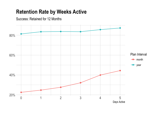
We see here that around 35% of monthly awesome customers were retained for 12 months, whereas around 85% of annual customers were retained for 12 months. Not bad!
Next we’ll do a bit of exploratory analysis to get a better understanding of the features we’re analyzing.
Exploratory Analysis
Let’s visualize the distribution of updates, profiles, days active, and weeks active for these users. We’ll begin with the number of days active during the first week on the plan (which can include the trial). Active is defined as creating at least one update with Buffer.
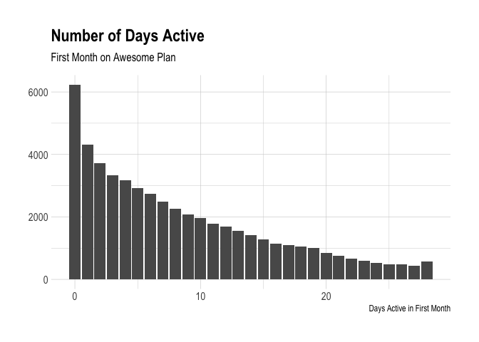
It’s interesting to see again that many users that were not active at all during their first four weeks on the plan! Our definition of “active” here is having scheduled at least one post with Buffer on any given day. We can see if this distribution looks different for users that were retained for four months versus those that were not.
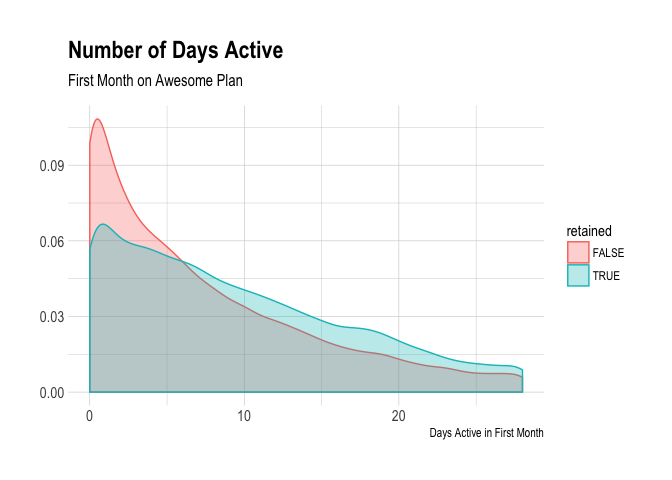
We can see that the distribution is skewed more to the left for folks that were not retained. A higher proportion of users were active for more days in the retained user population.
Let’s visualize the distribution of the number of weeks users are active in the first month. We’ll do this for both retained and churned users.
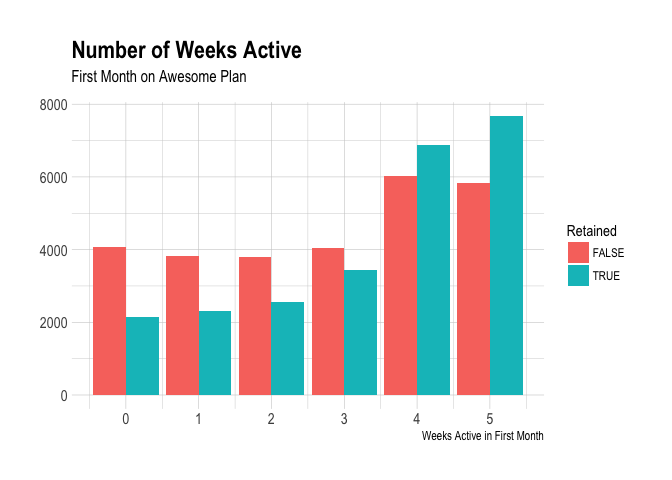
Cool, we can see that most users were active on four or five distince weeks! This is especially true of users that were retained for an year.
Next we’ll look at profiles. We’ll group profiles into these buckets and count how many users are in them:
- No profiles
- One profile
- Two to four profiles
- Five to eight profiles
- Nine or ten profiles
- 11+ profiles
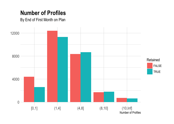
Interestingly, there are awesome customers that have no profiles after their first four weeks on the plan. The most common group is the one in which users have 2 to 4 profiles. For users that were retained for a year, the distribution is skewed slightly to the right.
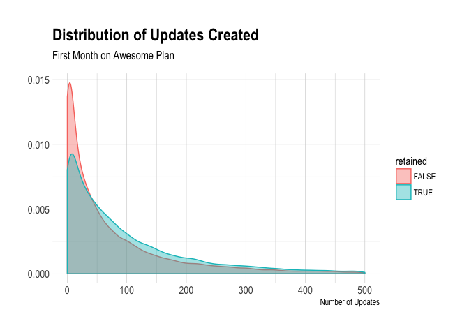
Moving on, we will look at the distribution of the number of updates awesome users created in their first month on the plan. Most users create low number of updates, but there is a long tail of users that create large numbers of updates during their first month on the awesome plan. We can see that retained users have tended to create more updates in their first month on the plan.
We can calculate the 99th percentile for updates again, in case there are outliers.
# get quantiles
quantile(awesome$updates, probs = c(0.25, 0.5, 0.75, 0.9, 0.99))
##    25%    50%    75%    90%    99%
##   12.0   51.0  135.0  294.0 1207.7
The 90th percentile is 294 updates and the 99th is 1208! We might remove users that have created 1500 or more updates in their first week and assume that these are outliers.
# remove potential outliers
awesome <- awesome %>%
  filter(updates < 1500)
Now, we can visualize the distribution of updates per profile to control for the fact that some users have many more profiles than others. I imagine that this distribution will have a similar shape to the one above, but let’s see…
# calculate updates per profile
awesome <- awesome %>%
  mutate(updates_per_profile = ifelse(is.na(profiles), 0, updates / profiles))
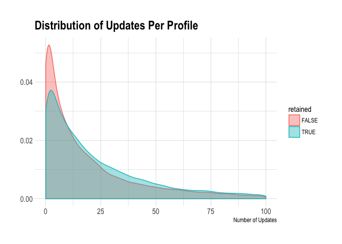
Right, we can see that the distributions are similar. The users that were retained scheduled slightly more updates per profile. Let’s see how having a trial associated with the subscription could affect the rate at which customers are retained for a year.
# get retention rates by trial
awesome %>%
  group_by(had_trial, retained) %>%
  summarise(users = n_distinct(user_id)) %>%
  mutate(percent = users / sum(users)) %>%
  filter(retained)
## # A tibble: 2 x 4
## # Groups:   had_trial [2]
##   had_trial retained users percent
##   <lgl>     <lgl>    <int>   <dbl>
## 1 F         T        23386   0.493
## 2 T         T         1432   0.493
We can see that having a trial associated with the subscription makes virtually no difference - the proportion of users that were retained for a year is virtually the same.
Calculating Correlations
Let’s run a logistic regression model to see how these features correlate with a user being retained for 12 months. We will control for the billing interval and normalize the features
# filter out annual plans
awesome <- awesome %>%
  mutate(profiles_scaled = scale(profiles),
         updates_per_profile_scaled = scale(updates_per_profile),
         updates_scaled = scale(updates))

# build model
mod <- glm(retained ~ profiles_scaled + updates_scaled + days_active + weeks_active + billing_interval +
            had_trial, data = awesome, family = 'binomial')

# summarise model
summary(mod)
##
## Call:
## glm(formula = retained ~ profiles_scaled + updates_scaled + days_active +
##     weeks_active + billing_interval + had_trial, family = "binomial",
##     data = awesome)
##
## Deviance Residuals:
##     Min       1Q   Median       3Q      Max
## -2.4074  -0.9206  -0.6944   0.7553   1.7553
##
## Coefficients:
##                       Estimate Std. Error z value Pr(>|z|)
## (Intercept)          -1.216150   0.023506 -51.738  < 2e-16 ***
## profiles_scaled       0.055033   0.010266   5.361 8.30e-08 ***
## updates_scaled        0.002322   0.012432   0.187    0.852
## days_active           0.011922   0.002548   4.679 2.88e-06 ***
## weeks_active          0.141870   0.009857  14.393  < 2e-16 ***
## billing_intervalyear  2.407792   0.026152  92.069  < 2e-16 ***
## had_trialTRUE         0.053045   0.043167   1.229    0.219
## ---
## Signif. codes:  0 '***' 0.001 '**' 0.01 '*' 0.05 '.' 0.1 ' ' 1
##
## (Dispersion parameter for binomial family taken to be 1)
##
##     Null deviance: 72347  on 52280  degrees of freedom
## Residual deviance: 59523  on 52274  degrees of freedom
## AIC: 59537
##
## Number of Fisher Scoring iterations: 4
The model output suggests that profiles, days, and weeks active are the features that have significant correlations with the likelihood of being retained for a year! We will examine all of these below.
Let’s begin by seeing how the number of days active affects the probability of beign retained.
Number of Days Active
We define a user as “active” on a day if he or she creates at least one update with Buffer on that day. Let’s look at the proportion of users that were retained for each number of days active in the first week on the awesome plan.
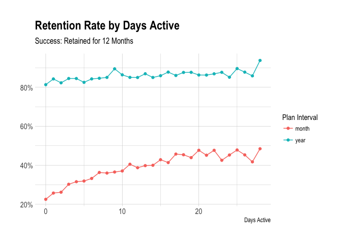
We can see the positive correlation between the number of days active and retention rates. The marginal differences are pretty linear though, so it’s not easy to find that inflection point, or “elbow”, that would serve as a good activation metric.
Again we see the small increases in the likelihood of being retained for every extra day active. As we’d excpect, there are some diminishing returns.
The marginal gain from an extra day active is quite small, but what if we looked at the number of weeks active instead of the number of days?
We see here that there is a nice increase in the proportion of users that were retained once they are active for four separate weeks. This could be of some use to us. Let’s move on to look at updates and profiles.
Updates and Profiles
We’ll use the same bucketing technique to see how the number of updates correlates with retention. The plot below shows the proportion of users in each update bucket that were retained for 12 months.
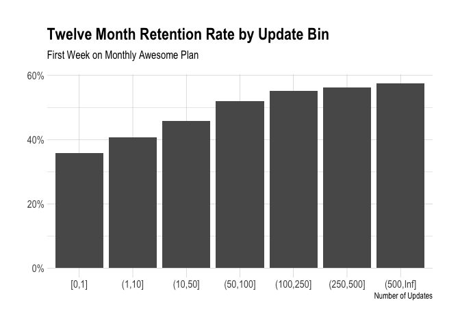
There is a significant bumps in the proportion of customers that are retained when one moves from 0 to 1, from 10 to 11, and from 50 to 51 updates. It might help to view the cumulative distribution function for this data.
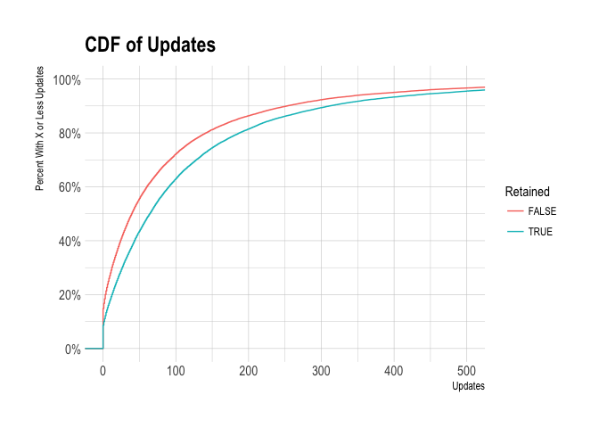
This graph shows us that customers that were retained for a year sent more updates in the 28 days. For example, around 58% of retained users sent 50 or more updates, whereas only around 44% of users that churned sent 50 or more updates.
Now let’s now look at updates per profile.
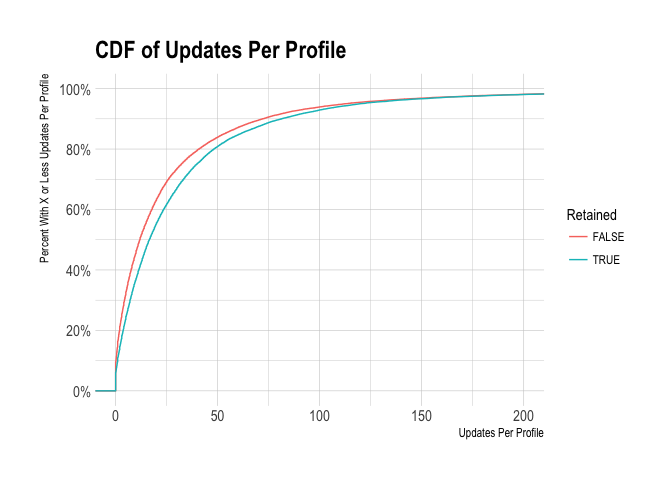
The cumulative distribution function (CDF) above shows us the percentage of customers with X or less updates per profile over the course of the 28 days. We can see that users that were retained for a year had slightly more - fore example, around 40% of retained users had more than 25 updates per profile, whereas around 30% of users that were not retained had more than 25 updates per profile.
We should also look at the number of profiles users have.
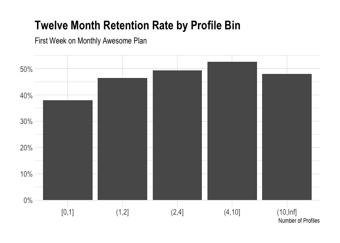
We can see a significant jump in retention when a user has more than one profile, but the gains after that initial jump are marginal.
Potential Activation Metrics
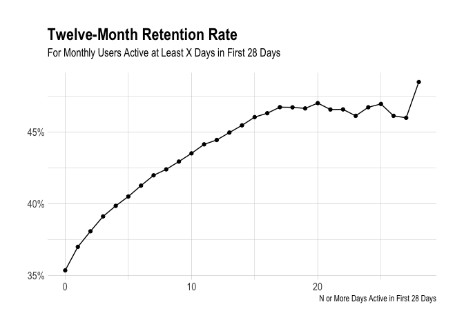
Let’s throw a few potential candidates at the wall and see what effect they’d have. We’ll start by defining “activated” as being not-inactive, i.e. at least one day active in the first week. What do retention rates look like for these people? For all of the potential activation metrics, we’ll look only at monthly customers. Annual customers are much more likely to be retained, so the effects of an activation metric can be more easily seen in monthly customers.
# one day active
awesome %>%
  filter(billing_interval == 'month') %>%
  group_by(not_inactive, retained) %>%
  summarise(users = n_distinct(user_id)) %>%
  mutate(percent = users / sum(users)) %>%
  filter(retained)
## # A tibble: 2 x 4
## # Groups:   not_inactive [2]
##   not_inactive retained users percent
##   <lgl>        <lgl>    <int>   <dbl>
## 1 F            T         1077   0.225
## 2 T            T        11717   0.370
If we define “activation” as having at least one day in which an update was created in the first 28 days, the likelihood of 12-month retention increases from around 23% to around 37%. Let’s look at two days active now.
# two days active
awesome %>%
  filter(billing_interval == 'month') %>%
  group_by(two_days, retained) %>%
  summarise(users = n_distinct(user_id)) %>%
  mutate(percent = users / sum(users)) %>%
  filter(retained)
## # A tibble: 2 x 4
## # Groups:   two_days [2]
##   two_days retained users percent
##   <lgl>    <lgl>    <int>   <dbl>
## 1 F        T         1939   0.240
## 2 T        T        10858   0.381
If we only require that a user be active for two or more days, then the retention rate increases from 24% to 38%. This return for requiring one extra day active is quite small. What if instead we required that users be active for multiple weeks?
# two weeks
awesome %>%
  filter(billing_interval == 'month') %>%
  group_by(two_weeks, retained) %>%
  summarise(users = n_distinct(user_id)) %>%
  mutate(percent = users / sum(users)) %>%
  filter(retained)
## # A tibble: 2 x 4
## # Groups:   two_weeks [2]
##   two_weeks retained users percent
##   <lgl>     <lgl>    <int>   <dbl>
## 1 F         T         2248   0.238
## 2 T         T        10549   0.388
If we rquire users to be active for at least two separate weeks, the proportion of users retained increases from 24% to 39%. We saw earlier that a higher percentage of users were retained if they had been active at least four weeks – what if we required that as an activation metric?
# four weeks
awesome %>%
  filter(billing_interval == 'month') %>%
  group_by(four_weeks, retained) %>%
  summarise(users = n_distinct(user_id)) %>%
  mutate(percent = users / sum(users)) %>%
  filter(retained)
## # A tibble: 2 x 4
## # Groups:   four_weeks [2]
##   four_weeks retained users percent
##   <lgl>      <lgl>    <int>   <dbl>
## 1 F          T         5312   0.276
## 2 T          T         7483   0.428
The proportion of users retained for a year increases from 28% to 43%. This is a nice increase of around 15%. We could look at updates instead – if we required at least 50 updates in the first 28 days, we’d see this.
# 50 updates
awesome %>%
  filter(billing_interval == 'month') %>%
  group_by(fifty_updates, retained) %>%
  summarise(users = n_distinct(user_id)) %>%
  mutate(percent = users / sum(users)) %>%
  filter(retained)
## # A tibble: 2 x 4
## # Groups:   fifty_updates [2]
##   fifty_updates retained users percent
##   <lgl>         <lgl>    <int>   <dbl>
## 1 F             T         5402   0.287
## 2 T             T         7395   0.414
The percentage of customers retained would increase from 29% to 41%. What if we required four weeks of activity and 10 updates?
# 10 updates 4 weeks
awesome %>%
  filter(billing_interval == 'month') %>%
  group_by(ten_updates_four_weeks, retained) %>%
  summarise(users = n_distinct(user_id)) %>%
  mutate(percent = users / sum(users)) %>%
  filter(retained)
## # A tibble: 2 x 4
## # Groups:   ten_updates_four_weeks [2]
##   ten_updates_four_weeks retained users percent
##   <lgl>                  <lgl>    <int>   <dbl>
## 1 F                      T         5343   0.276
## 2 T                      T         7452   0.428
The proportion of monthly customers retained for a year increases from 28% to 43%. This is what would occur if we required 50 updates.
# 50 updates 4 weeks
awesome %>%
  filter(billing_interval == 'month') %>%
  group_by(fifty_updates_four_weeks, retained) %>%
  summarise(users = n_distinct(user_id)) %>%
  mutate(percent = users / sum(users)) %>%
  filter(retained)
## # A tibble: 2 x 4
## # Groups:   fifty_updates_four_weeks [2]
##   fifty_updates_four_weeks retained users percent
##   <lgl>                    <lgl>    <int>   <dbl>
## 1 F                        T         6674   0.292
## 2 T                        T         6122   0.441
The proportion of users retained increases from 29% to 44%. Now let’s look at two weeks of activity and 50 updates.
# 50 updates 2 weeks
awesome %>%
  filter(billing_interval == 'month') %>%
  group_by(fifty_updates_two_weeks, retained) %>%
  summarise(users = n_distinct(user_id)) %>%
  mutate(percent = users / sum(users)) %>%
  filter(retained)
## # A tibble: 2 x 4
## # Groups:   fifty_updates_two_weeks [2]
##   fifty_updates_two_weeks retained users percent
##   <lgl>                   <lgl>    <int>   <dbl>
## 1 F                       T         5519   0.286
## 2 T                       T         7278   0.418
The proportion of monthly customers retained for a year would increase from 29% to 42%. What if we required 100 updates and two weeks of activity?
# 100 updates 2 weeks
awesome %>%
  filter(billing_interval == 'month') %>%
  group_by(hundred_updates_two_weeks, retained) %>%
  summarise(users = n_distinct(user_id)) %>%
  mutate(percent = users / sum(users)) %>%
  filter(retained)
## # A tibble: 2 x 4
## # Groups:   hundred_updates_two_weeks [2]
##   hundred_updates_two_weeks retained users percent
##   <lgl>                     <lgl>    <int>   <dbl>
## 1 F                         T         7948   0.313
## 2 T                         T         4847   0.431
The proportion of users retained increases from 32% to 43%. Now, what if we required 100 updates and 4 weeks of activity?
# 100 updates 4 weeks
awesome %>%
  filter(billing_interval == 'month') %>%
  group_by(hundred_updates_four_weeks, retained) %>%
  summarise(users = n_distinct(user_id)) %>%
  mutate(percent = users / sum(users)) %>%
  filter(retained)
## # A tibble: 2 x 4
## # Groups:   hundred_updates_four_weeks [2]
##   hundred_updates_four_weeks retained users percent
##   <lgl>                      <lgl>    <int>   <dbl>
## 1 F                          T         8474   0.314
## 2 T                          T         4321   0.450
The proportion increases from 31% to 45%.
Initial Conclusions
Of the potential activation metrics we examined, two weeks of activity, four weeks of activity, and four weeks of activity and at least 10 updates seem to have the highest potential return, around 15% increase in the likelihood of being retained for a full year.