Effect of Awesome/Pro Price Change
TL;DR
On March 22, 2018 we renamed the Awesome Plan to the Pro Plan, and changed its price from $10/mo to $15/mo. We announced the change and offered a promotion to let users lock in the $10/mo. price one month earlier, on February 22.
The effect of the price change is an increase of around $1500 in weekly MRR growth for Awesome/Pro plans. In the weeks prior to the price change announcement, MRR grew at an average rate of around $500 per week. In the weeks following the price change, Awesome/Pro MRR has grown at an average rate of around $2000 per week. The probability of a true causal effect is over 99% and the estimated effect size is around 300%!
In this analysis we’ll analyze the effect that the price change has had on MRR. We’ll utilize the Causal Impact package to estimate what MRR would have been without the price change and calculate the effect size from there. It’s important to note that the effect of the annual plan promotion likely interacts with the effect of the price change, so any effect on MRR will have come as a result of both events.
Data Collection
We’re estimating the effect that these changes had on MRR, so we’ll need to gather the subscriptions that contributed to Awesome/Pro MRR since January 1, 2018. We’ll use the data from this look and import it into our R session.
# get data from look
pro_mrr <- get_look(4466)
Great, we have the weekly MRR values for all of the Awesome and Pro Stripe plans from the past six months.
Exploratory Analysis
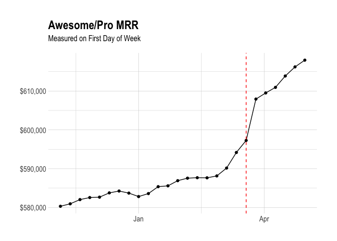
Let’s quickly visualize Awesome/Pro MRR over time. We’ll indicate the point at which the pricing changes took effect (the week of March 19).
We can see pretty clearly that there was a substantial effect on Awesome/Pro MRR in March. My hypothesis is that the offer to secure lower prices by subscribing to an annual Awesome plan resulted in a large, one-time effect, and that the Pro plan price change resulted in a smaller, long-term effect on MRR.
Let’s plot weekly MRR growth over time to see how it has changed.

We can see relatively steady MRR growth less than $1000 per week before March. After the price change announcement was made on February 22, we see a large increase in MRR growth and a relatively steady growth of around $2000 per week starting in April.
For reference, Business MRR grows around $2700 per week on average.
Measuring the Effect on MRR Growth
We’ll use a technique called Causal Impact for causal inference. Essentially, we take the weekly MRR change before the pricing change and forecast it into the future, and compare the forecast with the observed values. The difference between the counterfactual (what MRR growth would have happened without the pricing change) and the observed weekly MRR growth numbers is our estimated effect size.
We’ll also try to isolate the effect of the price change by excluding the weeks during which the promotional offer had a large effect. We do this by defining the “post-intervention period” as the weeks from April 2 onwards.
The “pre-intervention period”” includes weeks from November 13, 2017 to the week of February 26, which is the week that we announced the price change and the offer to lock in the lower prices. We use the average MRR growth from the weeks in the pre-intervention period to create our forecast of what MRR growth would have looked like without the pricing change. In this case, the simple average of $494 per week is used.
You’ll notice that we’ve left out a few weeks in March. The weeks of March 19 and March 26 saw unusually high MRR growth, and it’s my assumption is that this was primarily due to our offer to let users lock in the lower prices. We’ll use the weeks outside of this time window for our analysis.
To perform inference, we run the analysis using the CausalImpact command.
# run analysis
impact <- CausalImpact(mrr_ts, pre.period, post.period, model.args = list(niter = 5000))

# plot impact
plot(impact) +
  labs(title = "Impact on Awesome/Pro MRR") +
  scale_y_continuous(labels = dollar)
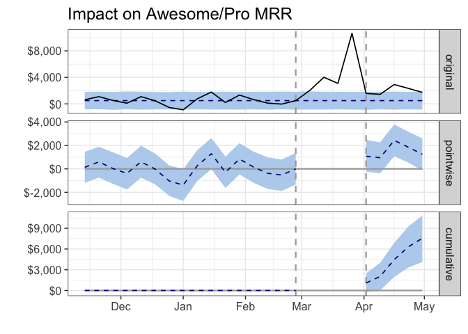
The pre-intervention period includes all data to the left of the first vertical dotted line, and the post-intervention period includes all data to the right of the second vertical dotted line.
The top panel in the graph shows the actual observed data (the black line) as well as the counterfactual, which is our best guess at what weekly MRR growth would have been had we not introduced a new plan.
The second panel displays the estimated effect that the price change had on MRR growth each week, and the bottom panel shows the cumulative effect over time on weekly MRR growth.
We can see that there was a big jump in weekly MRR growth during the month of March, mostly due to our offer to lock in the old prices, and a smaller increase in weekly MRR growth in the following weeks. Let’s calculate the exact difference and see if it is statistically significant.
# get summary
summary(impact)
## Posterior inference {CausalImpact}
##
##                          Average        Cumulative
## Actual                   2006           10030
## Prediction (s.d.)        494 (341)      2471 (1706)
## 95% CI                   [-162, 1183]   [-809, 5914]
##
## Absolute effect (s.d.)   1512 (341)     7559 (1706)
## 95% CI                   [823, 2168]    [4116, 10838]
##
## Relative effect (s.d.)   306% (69%)     306% (69%)
## 95% CI                   [167%, 439%]   [167%, 439%]
##
## Posterior tail-area probability p:   2e-04
## Posterior prob. of a causal effect:  99.97996%
##
## For more details, type: summary(impact, "report")
The probability of a true causal effect is over 99%. Average weekly MRR growth for the Awesome plans was $495 per week before the week of February 26, and $1986 per week for the weeks following March 26. This equates to an increase of around $1492 per week, an relative effect of over 300%!
This is an exciting trend, but we should remember that the promotional offer likely plays some role and that there will be a period of time in which the value of a new Pro customer gained (15/mo) is higher than the expected value of a churned customer (10/mo).
Also, we still have a relatively small sample size. The lower bound of the 95% confidence interval could perhaps be considered a conservative estimate of the effect size. The lower bound is an increase of $824 per week, or a relative increase of 67%.
Effect on Annual Subscriptions
Another change we made was to the relative discount of annual plans. The discount used to be 15% – with the new price change, the relative discount increased to 20%. The price of an annual Pro plan is $144. Did this change have any effect on the proportion of subscriptions that are billed annually? Let’s check!
select
  s.id as subscription_id
  , s.customer as customer_id
  , date(s.start) as start_date
  , date(date_trunc('week', s.start)) as start_week
  , date(s.canceled_at) as end_date
  , s.plan_id
  , p.billing_interval
  , count(distinct c.id) as successful_charges
from stripe._subscriptions as s
inner join stripe._invoices as i on i.subscription_id = s.id and s.plan_id = i.subscription_plan_id
inner join stripe._charges as c on c.invoice = i.id and c.captured and c.refunded = false
inner join dbt.plans as p on p.id = s.plan_id
where s.plan_id in ('pro-monthly', 'pro-annual',
  'pro_v1_monthly', 'pro_v1_yearly',
  'business_v2_small_monthly', 'business_v2_small_yearly')
and s.start >= '2017-08-01'
group by 1, 2, 3, 4, 5, 6, 7
Let’s calculate the percentage of subscriptions that are billed annually, for each week.
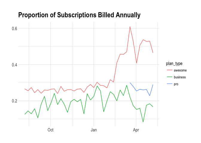
We can see the effect of the promotion again. Let’s only look at Awesome subscriptions started before February 22, 2018.
# get percentage of awesome subs
subs %>%
  filter(plan_type == 'awesome' & start_date < '2018-02-22') %>%
  group_by(billing_interval) %>%
  summarise(subs = n_distinct(subscription_id)) %>%
  mutate(percent = subs / sum(subs)) %>%
  filter(billing_interval == 'year')
## # A tibble: 1 x 3
##   billing_interval  subs percent
##   <chr>            <int>   <dbl>
## 1 year              7374   0.269
Around 27% of Awesome subscriptions started were billed annually. What about the Pro plans?
# get percentage of pro subs
subs %>%
  filter(plan_type == 'pro') %>%
  group_by(billing_interval) %>%
  summarise(subs = n_distinct(subscription_id)) %>%
  mutate(percent = subs / sum(subs)) %>%
  filter(billing_interval == 'year')
## # A tibble: 1 x 3
##   billing_interval  subs percent
##   <chr>            <int>   <dbl>
## 1 year              1243   0.261
A similar percentage, around 26%, of Pro subscriptions created are billed annually. Let’s compare this to the higher-priced small business plan.
# get percentage of pro subs
subs %>%
  filter(plan_type == 'business') %>%
  group_by(billing_interval) %>%
  summarise(subs = n_distinct(subscription_id)) %>%
  mutate(percent = subs / sum(subs)) %>%
  filter(billing_interval == 'year')
## # A tibble: 1 x 3
##   billing_interval  subs percent
##   <chr>            <int>   <dbl>
## 1 year               701   0.188
Only around 19% of small business plans are billed annually. This makes sense, as the plan is more expensive. Perhaps it’s a good thing that the rate of annual plans is the same, given that the price is over 40% higher than the previous annual plan’s price.