Finding Business Activation
28 March, 2018
In a previous analysis we used some simple EDA techniques to explore “activation” for new Buffer users.
In this analysis, we’ll use a similar approach to explore what activation could look like for users that subscribe to Buffer’s Business plans. We’ll define success in this case as being retained – not cancelling the subscription – for at least 12 months.
The features we’ll analyze are:
- The number of days that the user was a Buffer user before starting the subscription.
- The number of profiles the user added by the end of their first week on the plan.
- The number of team members the user added in their first week on the plan.
- The number of updates per profile created during the first week on the plan.
- The number of composer sessions that occurred during the first week on the plan.
- The number of days active during the first week on the plan.
Let’s collect the data.
Data Collection
We’ll run the query below to collect the data we need. We only want to get Business customers that have paid us successfully and that were active at least 12 months ago. We don’t know if Business subscriptions that were started in the past year will be retained for 12 months or not.
with business_users as (
  select
    s.id as subscription_id
    , s.customer as customer_id
    , u.id as user_id
    , date(u.created_at) as signup_date
    , date(s.start) as started_at
    , date(s.canceled_at) as canceled_at
    , s.plan_id
    , p.billing_interval
    , date(min(c.created)) as first_charge_date
  from stripe._subscriptions as s
  inner join dbt.users as u on s.customer = u.billing_stripe_customer_id
  inner join stripe._invoices as i
    on i.subscription_id = s.id
    and s.plan_id = i.subscription_plan_id
  inner join stripe._charges as c on c.invoice = i.id
    and c.captured
    and c.refunded = false
  inner join dbt.plans as p on p.id = s.plan_id
  where p.simplified_plan_id = 'business'
  and s.start >= '2016-01-01' and s.start < '2017-03-01'
  group by 1, 2, 3, 4, 5, 6, 7, 8
)

select
  b.subscription_id
  , b.customer_id
  , b.user_id
  , b.signup_date
  , b.started_at
  , b.canceled_at
  , b.first_charge_date
  , b.plan_id
  , b.billing_interval
  , count(distinct up.id) as updates
  , count(distinct mc.composer_session_id) as composer_sessions
  , count(distinct p.id) as profiles
  , count(distinct oa.user_id) as team_members
  , count(distinct date(up.created_at)) as days_active
from business_users as b
left join dbt.profiles as p on b.user_id = p.user_id
  and datediff(day, b.started_at, p.created_at) < 7
left join dbt.updates as up on p.id = up.profile_id
  and (up.created_at >= b.started_at and datediff(day, b.started_at, up.created_at) < 7)
  and up.was_sent_with_buffer
  and up.status != 'failed'
  and up.client_id in (
      '5022676c169f37db0e00001c', -- API and Extension
      '4e9680c0512f7ed322000000', -- iOS App
      '4e9680b8512f7e6b22000000', -- Android App
      '5022676c169f37db0e00001c', -- Feeds
      '5022676c169f37db0e00001c', -- Power Scheduler
      '539e533c856c49c654ed5e47', -- Buffer for Mac
      '5305d8f7e4c1560b50000008'  -- Buffer Wordpress Plugin
      )
left join dbt.multiple_composer_updates as mc
  on mc.update_id = up.id
left join dbt.org_permissions as oa
  on oa.org_owner_user_id = b.user_id
  and oa.user_id != oa.org_owner_user_id
  and oa.profile_role_created_at >= b.started_at
  and datediff(day, b.started_at, oa.profile_role_created_at) < 7
group by 1, 2, 3, 4, 5, 6, 7, 8, 9
Great, we have around 5000 Business users to work with. We’ll want to add a column to indicate if the user was retained for more than 365 days.
# calculate subscription length
business <- business %>%
  mutate(days_on_plan = ifelse(is.na(canceled_at),
                               as.numeric(Sys.Date() - started_at),
                               as.numeric(canceled_at - started_at)))

# indicate if user was retained for a full year
business <- business %>%
  mutate(retained = days_on_plan > 365)
Now let’s calculate the proportion of customers that were retained for 12 months – we’ll segment by the billing interval because annual customers may be more or less likely to be retained.
# get retention rate
business %>%
  group_by(billing_interval, retained) %>%
  summarise(users = n_distinct(customer_id)) %>%
  mutate(percent = users / sum(users)) %>%
  filter(retained)
## # A tibble: 2 x 4
## # Groups:   billing_interval [2]
##   billing_interval retained users percent
##   <chr>            <lgl>    <int>   <dbl>
## 1 month            T         1762   0.479
## 2 year             T         1077   0.910
We see here that around 48% of monthly business customers were retained for 12 months, whereas around 91% of annual customers were retained for 12 months. Not bad!
Next we’ll do a bit of exploratory analysis to get a better understanding of the features we’re analyzing.
Exploratory Analysis
Let’s visualize the distribution of updates, profiles, team members, days active, and composer sessions.
Days Active
We’ll begin with the number of days active during the first week on the plan (including the trial). Active here is defined as creating at least one update with Buffer.
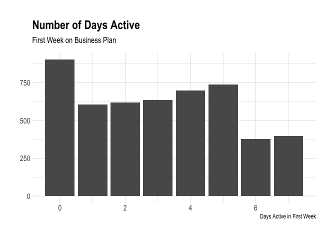
It’s striking to see again that many users that were not active at all during their first week on the plan! Our definition of “active” here is having scheduled at least one post with Buffer on any given day. It’s also interesting to note the decline once we reach six days – I suspect that the five-day workweek might have something to do with this characteristic. Let’s view the distribution for both retained and non-retained users.
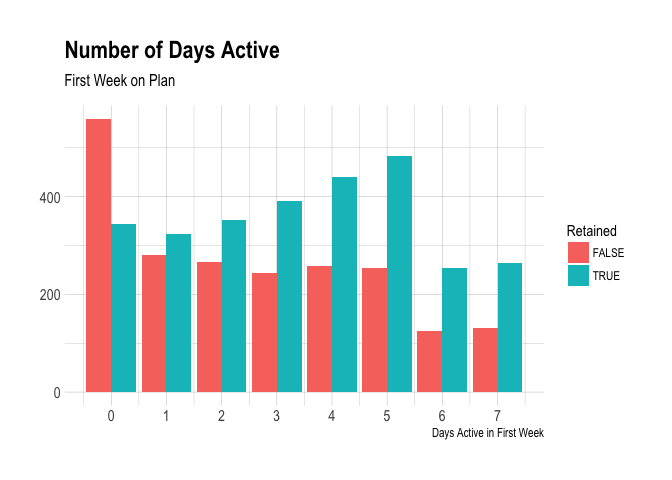
Cool, we can see that the distribution is shifted to the right for users that were retained for 12 months. Next we’ll look at profiles.
Profiles
We’ll group profiles into these buckets and count how many users are in them:
- No profiles
- One profile
- Two to five profiles
- Six to ten profiles
- 11-25 profiles
- 26+ profiles
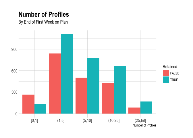
Interestingly, there are Business customers that have no profiles after their first week on the plan. I’m not sure what’s going on there. The most common group is the one in which users have 2 to 5 profiles, which is interesting.
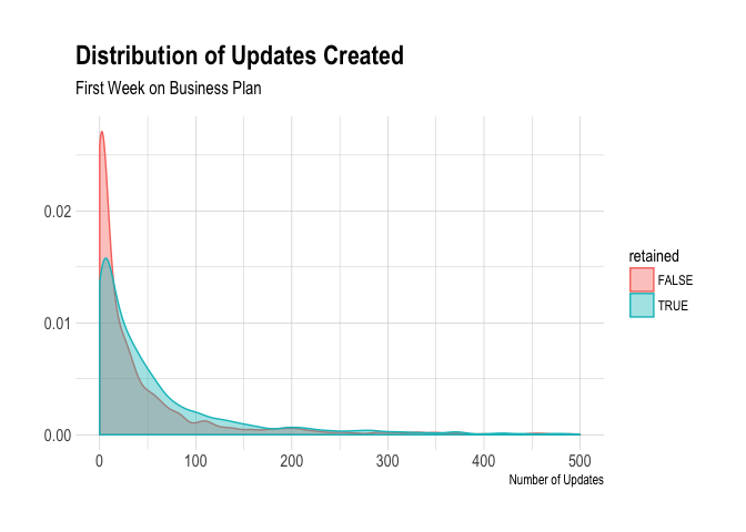
Moving on, we will look at the distribution of the number of updates Business users created in their first week on the plan.
Updates
This is the type of distribution we’d expect to see. Most users create low number of updates, but there is a long tail of users that create many updates during their first week on the Business plan. We can see that retained users have tended to create more updates in their first week on the plan.
We can calculate the 99th percentile for updates again, in case there are outliers.
# get quantiles
quantile(business$updates, probs = c(0.25, 0.5, 0.75, 0.9, 0.99))
##     25%     50%     75%     90%     99%
##    4.00   23.00   66.00  185.30 1380.32
The 90th percentile is 185 updates and the 99th is 1380 updates created in the first week, so we might remove users that have created 1000 or more updates in their first week and assume that these are outliers.
# remove potential outliers
business <- business %>%
  filter(updates < 1000)
We should also visualize the distribution of updates per profile to control for the fact that some users have many more profiles than others. I imagine that this distribution will have a similar shape to the one above, but let’s see…
# calculate updates per profile
business <- business %>%
  mutate(updates_per_profile = ifelse(is.na(profiles), 0, updates / profiles))
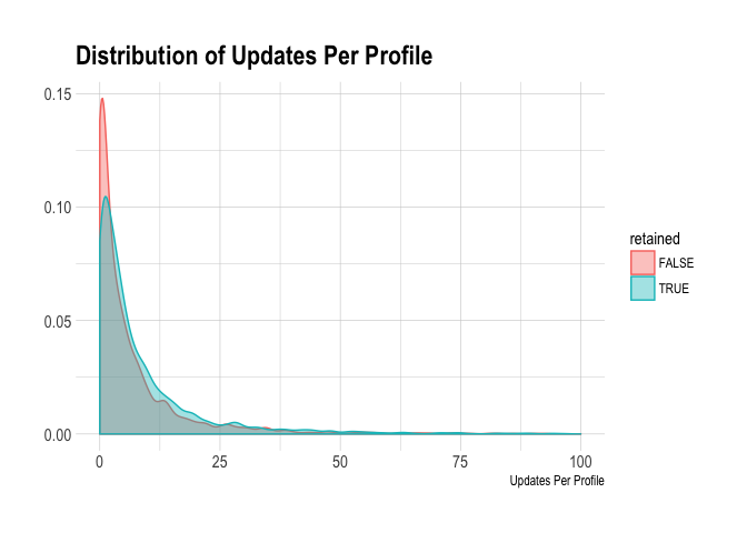
Right, we can see that the distributions are similar. A bit later we’ll look at how the number of updates correlates with the likelihood of being retainted, but for now let’s look at the distribution of team members.
Team Members
We’ll use the same technique of “bucketing” the team member counts.
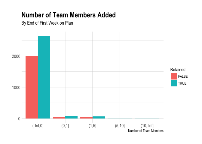
We can see that the biggest bucket by far is the one in which users have no team members. It does seem like users that were retained were more likely to have team members.
Calculating Correlations
Let’s run a logistic regression model to see how these features correlate with a user being retained for 12 months. We will control for the billing interval and normalize some of the features. Instead of using the number of team members as a feature, we will create a boolean variable that indicates whether or not a user had a team member.
# filter out annual plans
business <- business %>%
  mutate(profiles_scaled = scale(profiles),
         updates_scaled = scale(updates),
         composer_sessions_scaled = scale(composer_sessions),
         has_team_member = team_members > 0)

# build model
mod <- glm(retained ~ profiles_scaled + updates_scaled + days_active + billing_interval +
             has_team_member, data = business, family = 'binomial')

# summarise model
summary(mod)
##
## Call:
## glm(formula = retained ~ profiles_scaled + updates_scaled + days_active +
##     billing_interval + has_team_member, family = "binomial",
##     data = business)
##
## Deviance Residuals:
##     Min       1Q   Median       3Q      Max
## -2.6881  -1.0207   0.3747   1.0812   1.5420
##
## Coefficients:
##                      Estimate Std. Error z value Pr(>|z|)
## (Intercept)          -0.72372    0.06124 -11.818  < 2e-16 ***
## profiles_scaled       0.18560    0.04056   4.576 4.75e-06 ***
## updates_scaled       -0.04272    0.03794  -1.126   0.2601
## days_active           0.19077    0.01682  11.340  < 2e-16 ***
## billing_intervalyear  2.48870    0.10735  23.184  < 2e-16 ***
## has_team_memberTRUE   0.29375    0.14939   1.966   0.0493 *
## ---
## Signif. codes:  0 '***' 0.001 '**' 0.01 '*' 0.05 '.' 0.1 ' ' 1
##
## (Dispersion parameter for binomial family taken to be 1)
##
##     Null deviance: 6682.7  on 4897  degrees of freedom
## Residual deviance: 5655.3  on 4892  degrees of freedom
## AIC: 5667.3
##
## Number of Fisher Scoring iterations: 5
The model output suggests that the number of profiles, the number of days active, whether or not a user has a team member, and the billing interval all have significant correlations with the likelihood of being retained for a year. We’ll examine each of these in more detail below.
We’ll start by seeing how the number of days active affects the probability of beign retained.
Number of Days Active
We define a user as “active” on a day if he or she creates at least one update with Buffer on that day. Let’s look at the proportion of users that were retained for each number of days active in the first week on the Business plan.
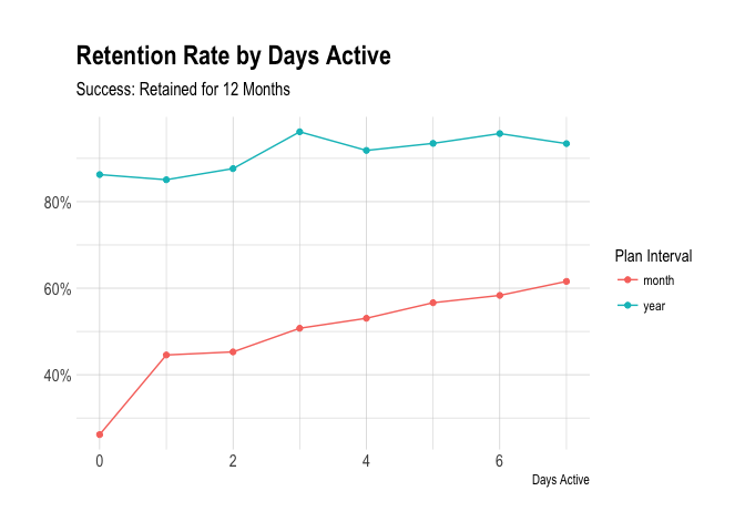
We can see the positive correlation between the number of days active and retention rates. The marginal differences are relatively small though - the biggest increase comes from zero to one. We definitely don’t want business users to be inactive! The marginal increase for monthly users is mostly linear from 2 to 7 days, but there is a local maximum at 3 days for yearly customers.
Below we’ll examine the increase in the “success rate” for users that were active X or more days in their first week on the plan. We’ll only look at monthly customers, as an effect will likely be easier to tease out.
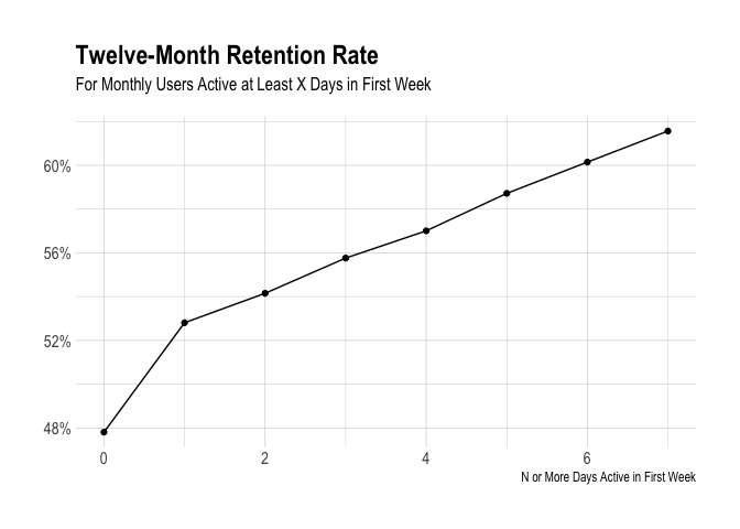
We can see here that the biggest jump comes from being active at least one day. From one to seven days, the increase in retention rates seems to be linear. Naturally, users that are active every day have the highest chance of being retained for twelve months.
Next we’ll examine profiles and updates.
Updates and Profiles
We’ll use the same bucketing technique to see how the number of updates correlates with retention. The plot below shows the proportion of users in each update bucket that were retained for 12 months.
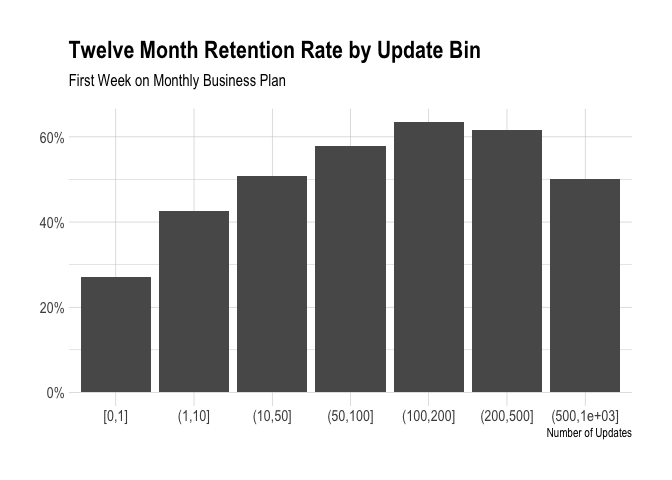
There is a significant bump when we move from 0 updates to 1-10. That makes sense - we’d prefer for Business customers not to be inactive during their first week on the plan. There seems to be a roughly linear increase in retention rates up to 100 updates.
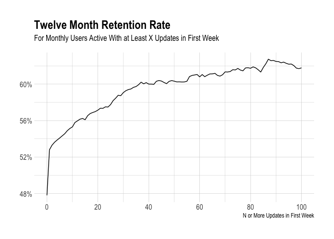
We can see here that there is a big jump from zero to one, and diminishing gains thereafter. What if we looked at the same chart, but for updates per profile instead of just the number of updates?
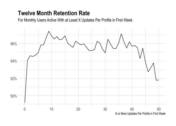
This is also interesting to see. The maximum seems to be around 8 updates per profile – beyond that there seem to be negative returns.
What at we looked at the number of composer sessions? A composer session is one in which updates are created and scheduled from the web or extension composer.
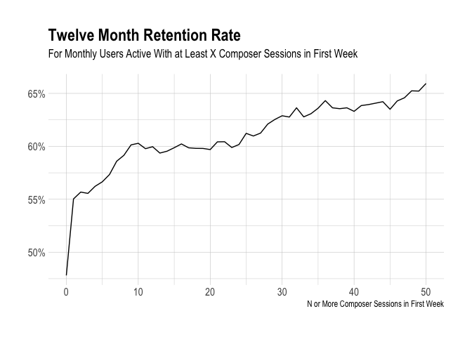
There does seem to be a positive correlation here, but the marginal difference that it makes is relatively small. It could possibly be worth looking into more.
We should also look at the number of profiles users have. We remember that this was one of the most significant positive correlations.
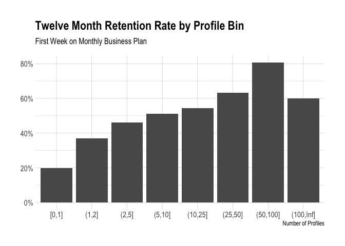
We can see a significant jump in retention when a user has more than one profile, but the gains after that initial jump are marginal.
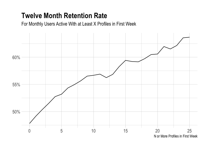
There doesn’t seem to be any inflection point or “elbow” here, but it could still be of some use to us. Perhaps we could look at something like 8 profiles.
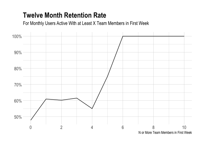
Team Members
Let’s see how the likelihood of retention correlates with the number of team members users have. Let’s start by looking at the proportion of users with at least one team member that were retained for a year.
# has team member
business %>%
  filter(billing_interval == 'month') %>%
  group_by(has_team_member, retained) %>%
  summarise(users = n_distinct(customer_id)) %>%
  mutate(percent = users / sum(users)) %>%
  filter(retained)
## # A tibble: 2 x 4
## # Groups:   has_team_member [2]
##   has_team_member retained users percent
##   <lgl>           <lgl>    <int>   <dbl>
## 1 F               T         1621   0.471
## 2 T               T          114   0.610
Around 47% of monthly business users without a team member were retained for a year, wheras around 61% of monthly business users with a team member were retained for a year.
Potential Activation Metrics
Let’s throw a few potential candidates at the wall and see what effect they’d have. For now we’ll only look at the effect on monthly business customers, since the effect is easier to tease out (remember around 90% of annual customers are retained).
We’ll start by defining “activated” as being not-inactive, i.e. at least one day active in the first week. What do retention rates look like for these people?
# one day active
business %>%
  filter(billing_interval == 'month') %>%
  group_by(not_inactive, retained) %>%
  summarise(users = n_distinct(user_id)) %>%
  mutate(percent = users / sum(users)) %>%
  filter(retained)
## # A tibble: 2 x 4
## # Groups:   not_inactive [2]
##   not_inactive retained users percent
##   <lgl>        <lgl>    <int>   <dbl>
## 1 F            T          186   0.262
## 2 T            T         1553   0.528
If we define “activation” as having at least one day in which an update was created in the first week, the likelihood of 12-month retention increases from around 26% to around 53% for monthly customers. Let’s look at two days active now.
# two days active
business %>%
  filter(billing_interval == 'month') %>%
  group_by(two_days, retained) %>%
  summarise(users = n_distinct(user_id)) %>%
  mutate(percent = users / sum(users)) %>%
  filter(retained)
## # A tibble: 2 x 4
## # Groups:   two_days [2]
##   two_days retained users percent
##   <lgl>    <lgl>    <int>   <dbl>
## 1 F        T          395   0.335
## 2 T        T         1344   0.542
If we only require that a user be active for two or more days, then the retention rate increases from 34% to 54% for monthly customers. This return for requiring one extra day active is quite small. What if we required two days of activity and a team member?
# two days active and one team member
business %>%
  filter(billing_interval == 'month') %>%
  group_by(two_days_one_team, retained) %>%
  summarise(users = n_distinct(user_id)) %>%
  mutate(percent = users / sum(users)) %>%
  filter(retained)
## # A tibble: 2 x 4
## # Groups:   two_days_one_team [2]
##   two_days_one_team retained users percent
##   <lgl>             <lgl>    <int>   <dbl>
## 1 F                 T         1641   0.470
## 2 T                 T           98   0.658
The likelihood of a monthly customer being retained increases from 47% to 65%, which is a pretty big increase! However, very few business customers seem to meet these criteria.
Next let’s see what happens if we require at least five composer sessions.
# five composer sessions
business %>%
  filter(billing_interval == 'month') %>%
  group_by(five_composer_sessions, retained) %>%
  summarise(users = n_distinct(user_id)) %>%
  mutate(percent = users / sum(users)) %>%
  filter(retained)
## # A tibble: 2 x 4
## # Groups:   five_composer_sessions [2]
##   five_composer_sessions retained users percent
##   <lgl>                  <lgl>    <int>   <dbl>
## 1 F                      T         1347   0.454
## 2 T                      T          392   0.566
The retention rate would increase from 45% to 57%. It seems that looking at the number of active days is more useful to us. Let’s see how these rates would change if we required 10 composer sessions.
# ten composer sessions
business %>%
  filter(billing_interval == 'month') %>%
  group_by(ten_composer_sessions, retained) %>%
  summarise(users = n_distinct(user_id)) %>%
  mutate(percent = users / sum(users)) %>%
  filter(retained)
## # A tibble: 2 x 4
## # Groups:   ten_composer_sessions [2]
##   ten_composer_sessions retained users percent
##   <lgl>                 <lgl>    <int>   <dbl>
## 1 F                     T         1402   0.452
## 2 T                     T          337   0.603
If we required 10 composer sessions, the likelihood of being retained for a year would increase from 45% to 60%. Again tt seems like one or two days active would be more appropriate. Now, what if we required at least 8 updates per profile to be created?
# eight updates per profile
business %>%
  filter(billing_interval == 'month') %>%
  group_by(eight_updates_per_profile, retained) %>%
  summarise(users = n_distinct(user_id)) %>%
  mutate(percent = users / sum(users)) %>%
  filter(retained)
## # A tibble: 3 x 4
## # Groups:   eight_updates_per_profile [3]
##   eight_updates_per_profile retained users percent
##   <lgl>                     <lgl>    <int>   <dbl>
## 1 F                         T         1120   0.455
## 2 T                         T          592   0.567
## 3 NA                        T           27   0.173
The retention rate increases from 46% to 57% – it seems like we don’t really need the condition on updates per profile. What if we required 10 updates overall and two days of activity?
# ten updates and two days of activity
business %>%
  filter(billing_interval == 'month') %>%
  group_by(ten_updates_two_days, retained) %>%
  summarise(users = n_distinct(user_id)) %>%
  mutate(percent = users / sum(users)) %>%
  filter(retained)
## # A tibble: 2 x 4
## # Groups:   ten_updates_two_days [2]
##   ten_updates_two_days retained users percent
##   <lgl>                <lgl>    <int>   <dbl>
## 1 F                    T          518   0.353
## 2 T                    T         1221   0.557
The liklihood of a monthly business customer being retained would increase from 35% to 56% – not too bad! Let’s look at what would happen if we only required 10 updates.
# ten updates
business %>%
  filter(billing_interval == 'month') %>%
  group_by(ten_updates, retained) %>%
  summarise(users = n_distinct(user_id)) %>%
  mutate(percent = users / sum(users)) %>%
  filter(retained)
## # A tibble: 2 x 4
## # Groups:   ten_updates [2]
##   ten_updates retained users percent
##   <lgl>       <lgl>    <int>   <dbl>
## 1 F           T          435   0.336
## 2 T           T         1304   0.553
Retention increases from 34% to 55%. That’s a pretty good return! Now let’s see what would happen if we also required one team member.
# ten updates and one team member
business %>%
  filter(billing_interval == 'month') %>%
  group_by(ten_updates_one_team, retained) %>%
  summarise(users = n_distinct(user_id)) %>%
  mutate(percent = users / sum(users)) %>%
  filter(retained)
## # A tibble: 2 x 4
## # Groups:   ten_updates_one_team [2]
##   ten_updates_one_team retained users percent
##   <lgl>                <lgl>    <int>   <dbl>
## 1 F                    T         1644   0.470
## 2 T                    T           95   0.693
The likelihood of being retained for a full year increases from around 47% to 69%! That is quite promising - the challenge is that very few users (around 4%) actually activate under those conditions. Let’s look at one more.
# ten updates and four profiles
business %>%
  filter(billing_interval == 'month') %>%
  group_by(ten_updates_four_profiles, retained) %>%
  summarise(users = n_distinct(user_id)) %>%
  mutate(percent = users / sum(users)) %>%
  filter(retained)
## # A tibble: 2 x 4
## # Groups:   ten_updates_four_profiles [2]
##   ten_updates_four_profiles retained users percent
##   <lgl>                     <lgl>    <int>   <dbl>
## 1 F                         T          613   0.363
## 2 T                         T         1126   0.574
Requiring four profiles and ten updates increases the retention rate from 36% to 57%.
Initial Conclusions
A user being active on more than one day of their first week on the plan has a higher chance of being retained long-term, but I would hesitate before saying that increasing the number of days that a user is active during their first week on the plan has a causal impact on retention.
The most promising activation metrics we could try, based on the data I’ve looked at so far, is requiring at least 10 updates over the course of two days to be created during users’ first week or requiring ten updates and at least one team member. This raises the probability of being retained by around 20%, but not many business customers “activate” under these definitions.