Equal Pay Report 2018
03 April, 2018
Last April we released Buffer’s first equal pay report in celebration of Equal Pay Day. Since then, we have overhauled our salary formula and made many internal role changes. Given all of these changes, I’m excited to dig into our salary data today and see how we’re doing.
Data Collection
The data we’ll use in this analysis comes from this spreadsheet. Let’s read the data into this R session and take a glimpe at what the data looks like.
# read csv
salaries <- read.csv("~/Downloads/salaries.csv", header = TRUE)
Now let’s do some exploratory analysis.
Summary Statistics
We will first average total cash compensation across the company, including base salary, dependent grants, and the salary/equity choice. We will break down how each component influences the wage gap later on.
To begin, let’s calculate the mean and median pay of employees of Buffer.
# find median and mean
salaries %>%
  summarise(average_pay = mean(salary), median_pay = median(salary))
##   average_pay median_pay
## 1    111832.6     106709
The average salary, including dependent grants and salary choice, is $111,832, and the median salary is $106,709. We can visualize what the distribution looks like with a histogram.
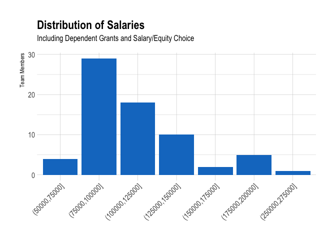
We can see that most team members fall within the $75,000 to $100,000 range.
Average Salary by Gender
Let’s calculate the average pay, including base salary, dependent grants, and salary/equity choice, for men and women at Buffer.
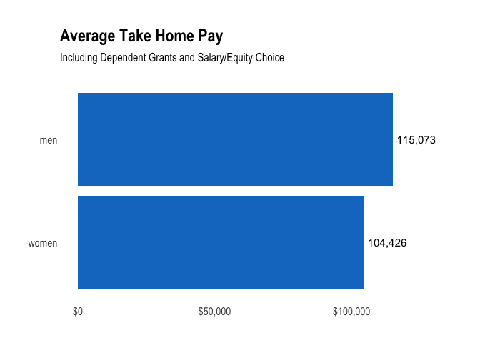
The average salary for men at Buffer is $115,073 and the average salary for women is $104,426. On average, across the entire team, men earn around 10% more than women. Let’s take a look at the distribution of salaries for men and women.
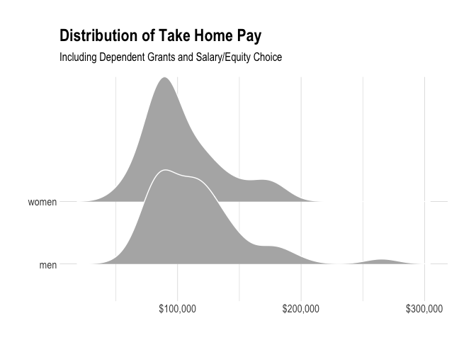
These distributions are useful to see. For women, the center of the distribution is centered slighly to the left, below $100,000, and is narrower. Men have a wider distribution, as there are more men in technical, higher-paying roles.
Average Salary by Role Type
Last year we saw an interesting example of Simpson’s Paradox. We saw that, across the entire team, men earned significantly more than women. However, when broken down into technical and non-technical roles, we saw that women earned more, on average, in each category.
Let’s break the average salary down by role type again. The three role types are technical (engineering, data, product, and design), non-technical (finance, marketing, advocacy, and people), and leadership.
tech <- salaries %>%
  filter(role_type == 'technical') %>%
  group_by(gender) %>%
  summarise(average_salary = mean(salary)) %>%
  ungroup() %>%
  ggplot(aes(x = gender, y = average_salary)) +
  geom_bar(stat = 'identity', fill = '#0366d6') +
  geom_text(aes(label = comma(round(average_salary, 0))), vjust = -1, size = 4) +
  theme_ipsum() +
  theme(panel.grid.major = element_blank(), panel.grid.minor = element_blank()) +
  scale_y_continuous(labels = dollar_format(), limits = c(0, 220000)) +
  labs(x = NULL, y = NULL, title = " ", subtitle = "Technical Roles")

nontech <- salaries %>%
  filter(role_type == 'non-technical' & team != 'leadership') %>%
 group_by(gender) %>%
  summarise(average_salary = mean(salary)) %>%
  ungroup() %>%
  ggplot(aes(x = gender, y = average_salary)) +
  geom_bar(stat = 'identity', fill = '#c75050') +
  geom_text(aes(label = comma(round(average_salary, 0))), vjust = -1, size = 4) +
  theme_ipsum() +
  theme(panel.grid.major = element_blank(), panel.grid.minor = element_blank()) +
  scale_y_continuous(labels = dollar_format(), limits = c(0, 220000)) +
  labs(x = NULL, y = NULL, title = " ", subtitle = "Non-Technical Roles")

leaders <- salaries %>%
  filter(team == 'leadership') %>%
  group_by(gender) %>%
  summarise(average_salary = mean(salary)) %>%
  ungroup() %>%
  ggplot(aes(x = gender, y = average_salary)) +
  geom_bar(stat = 'identity') +
  geom_text(aes(label = comma(round(average_salary, 0))), vjust = -1, size = 4) +
  theme_ipsum() +
  theme(panel.grid.major = element_blank(), panel.grid.minor = element_blank()) +
  scale_y_continuous(labels = dollar_format(), limits = c(0, 220000)) +
  labs(x = NULL, y = NULL, title = "Average Take Home Pay", subtitle = "Leadership Roles")

grid.arrange(leaders, tech, nontech, ncol = 3)
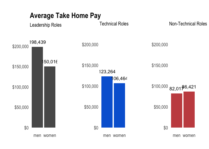
In technical roles, men earn around 16% more than women on average. In non-technical roles, women earn around 5% more than men. In leadership roles, men earn around 32% more than women on average.
Dependent Grants
Dependent grants can be thought of as a separate component of total cash compensation. We’ve decided to include it in this analysis in order to share as much information as possible, but we could have also left it out. Let’s explore what effect this component has on average pay for women and men. We can calculate what proportion of team members claim dependents.
# proportion that claim dependents
salaries %>%
  mutate(has_dependents = dependents > 0) %>%
  group_by(gender, has_dependents) %>%
  summarise(people = n()) %>%
  mutate(percent = people / sum(people))
## # A tibble: 4 x 4
## # Groups:   gender [2]
##   gender has_dependents people percent
##   <fct>  <lgl>           <int>   <dbl>
## 1 men    F                  18   0.375
## 2 men    T                  30   0.625
## 3 women  F                  15   0.714
## 4 women  T                   6   0.286
We see that 63% of men claim at least one dependent, compared to 29% of women. In Buffer, men are more than twice as likely as women to claim dependents.
# find average number of dependents claimed
salaries %>%
  filter(dependents > 0) %>%
  group_by(gender) %>%
  summarise(avg_dependends = mean(dependents))
## # A tibble: 2 x 2
##   gender avg_dependends
##   <fct>           <dbl>
## 1 men              1.97
## 2 women            2.50
Of those people that claim dependents, men claim an average of 2, and women claim an average of 2.5. Let’s see how this component affects average salaries.
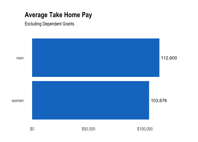
The average salary for men, excluding dependent grants, is around 9% higher than that of women.
Salary Choice
Back in 2013, we began offering teammates the option between an additional $10,000 in annual salary or accepting 30% more in stock options. Around 71% of our current team opted to take the higher salary choice. Let’s see how this breaks down for men and women.
# proportion that took salary choice
salaries %>%
  mutate(took_salary_choice = salary_choice > 0) %>%
  group_by(gender, took_salary_choice) %>%
  summarise(people = n()) %>%
  mutate(percent = people / sum(people))
## # A tibble: 4 x 4
## # Groups:   gender [2]
##   gender took_salary_choice people percent
##   <fct>  <lgl>               <int>   <dbl>
## 1 men    F                      18   0.375
## 2 men    T                      30   0.625
## 3 women  F                       6   0.286
## 4 women  T                      15   0.714
Around 63% of men benefit from the salary choice, compared to around 71% of women on the team. Let’s see how average salaries would look if we removed both the salary choice and dependent grants.
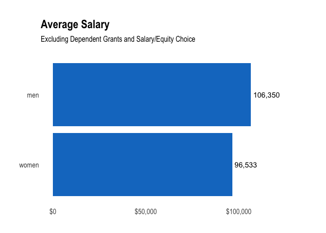
If we remove dependent grants and the salary/equity choice and only look at base salary, men still earn around 10% more than women on average.
Location
The location multiplier makes a large difference in salaries. Let’s see how it affects men and women on the team.
# proportion that took salary choice
salaries %>%
  group_by(gender, location_multiplier) %>%
  summarise(people = n()) %>%
  mutate(percent = people / sum(people))
## # A tibble: 6 x 4
## # Groups:   gender [2]
##   gender location_multiplier people percent
##   <fct>                <int>  <int>   <dbl>
## 1 men                     75      2  0.0417
## 2 men                     85     37  0.771
## 3 men                    100      9  0.188
## 4 women                   75      1  0.0476
## 5 women                   85     19  0.905
## 6 women                  100      1  0.0476
Around 5% of women have the lowest location multiplier of 0.75, 90% have a location multiplier of 0.85, and 5% have the highest location multiplier of 1.
This is substantially different than the distribution for men: around 4% have the lowest multiplier, 77% have the middle multiplier of 0.85, and 19% have the highest location multiplier of 1.
Here is what the average salaries would be if we controlled for location.
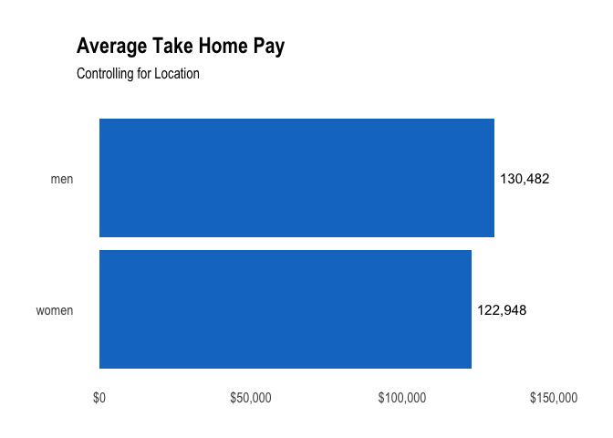
If we control for the differences in location, men still earn around 6% more than women on average.
Salaries by Team
We can also plot the average salary for each team at Buffer.
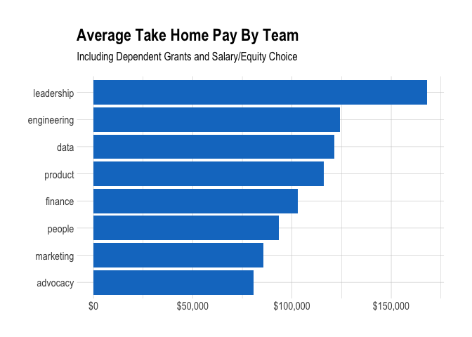
This is an interesting graph to look at, but let’s breakdown the average salaries for each team.
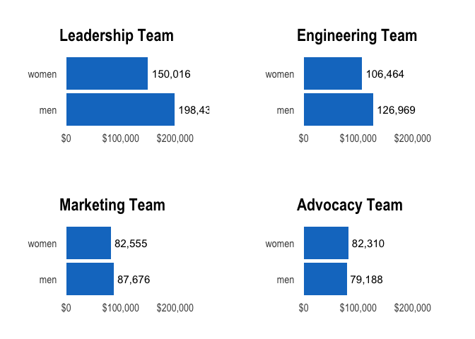
We can break this down by team. The product, data, and design teams consist only of men. The finance and people teams consist only of women. Interesting stuff overall! We still have some work to do.