Defining an Activation Rate
28 March, 2018
A couple years ago we found that new users were more likely to be successful with Buffer if they scheduled at least three updates in their first seven days after signing up. We defined success as still being an active user three months after signing up.
In this analysis we’ll revisit the assumptions we made and determine if this “three updates in seven days” activation metric is still appropriate. To do that, we’ll examine usage in the first week after signing up for Buffer. We’ll look at the number of posts scheduled, the number of profiles added, and the number of days that users were active. We will again define success as being retained for three months.
Based on some basic exploratory analysis below, I might suggest an activation metric of at least three days active within the first week. Using this definition, approximately 15% of new users end up activating.
Around 26% of users that did not activate were retained for three months, whereas 52% of users that activated were retained. Activated users are twice as likely to be retained for three months by this definition.
Data Collection
We’ll want to gather all users that signed up before three months ago. We don’t yet know if users that signed up in the past three months were “successful” or not. We also want to know how many profiles they added in the first week and how many updates were created. We want users that signed up between December 1, 2016 and December 1, 2017.
We’ll gather that data with the following query.
with last_active_date as (
  select
    user_id
    , max(date(created_at)) as last_active_date
  from dbt.updates
  where was_sent_with_buffer
  and status != 'failed'
  and created_at > '2016-12-01'
  and client_id in (
        '5022676c169f37db0e00001c', -- API and Extension
        '4e9680c0512f7ed322000000', -- iOS App
        '4e9680b8512f7e6b22000000', -- Android App
        '5022676c169f37db0e00001c', -- Feeds
        '5022676c169f37db0e00001c', -- Power Scheduler
        '539e533c856c49c654ed5e47', -- Buffer for Mac
        '5305d8f7e4c1560b50000008'  -- Buffer Wordpress Plugin
        )
  group by 1
)

select
  u.id as user_id
  , date(u.created_at) as signup_date
  , l.last_active_date
  , count(distinct p.id) as profiles
  , count(distinct up.id) as updates
  , count(distinct date(up.created_at)) as days_active
from dbt.users as u
left join dbt.profiles as p
  on u.id = p.user_id and datediff(day, u.created_at, p.created_at) < 7
left join dbt.updates as up
  on p.id = up.profile_id
  and up.was_sent_with_buffer
  and datediff(day, u.created_at, up.created_at) < 7
  and status != 'failed'
  and client_id in (
        '5022676c169f37db0e00001c', -- API and Extension
        '4e9680c0512f7ed322000000', -- iOS App
        '4e9680b8512f7e6b22000000', -- Android App
        '5022676c169f37db0e00001c', -- Feeds
        '5022676c169f37db0e00001c', -- Power Scheduler
        '539e533c856c49c654ed5e47', -- Buffer for Mac
        '5305d8f7e4c1560b50000008'  -- Buffer Wordpress Plugin
        )
inner join last_active_date as l on u.id = l.user_id
where u.created_at >= '2016-12-01' and u.created_at <= '2017-12-01'
group by 1, 2, 3
Great, we now have around 670 thousand Buffer users to analyze!
Data Tidying
We want to know if the user was successful. We do this by determining if the user was still active 90 days after signing up. If the user didn’t send any updates, we’ll set their last_active_date to the signup_date value.
# set last active date
users$last_active_date[is.na(users$last_active_date)] <- users$signup_date

# determine if user was successful
users <- users %>%
  mutate(successful = as.numeric(last_active_date - signup_date) >= 90)
Let’s see what proportion of signups were retained for three months.
# get success rate
users %>%
  group_by(successful) %>%
  summarise(users = n_distinct(user_id)) %>%
  mutate(percent = users / sum(users))
## # A tibble: 2 x 3
##   successful  users percent
##   <lgl>       <int>   <dbl>
## 1 F          468505   0.703
## 2 T          197961   0.297
Around 30% of users were retained for three months or more.
Searching for Activation
Now let’s see how well these metrics correlate with success. To do so, we’ll use a logistic regression model.
# define logistic regression model
mod <- glm(successful ~ profiles + updates + days_active, data = users, family = "binomial")

# summarize the model
summary(mod)
##
## Call:
## glm(formula = successful ~ profiles + updates + days_active,
##     family = "binomial", data = users)
##
## Deviance Residuals:
##     Min       1Q   Median       3Q      Max
## -5.3890  -0.8110  -0.7689   1.4096   1.7063
##
## Coefficients:
##               Estimate Std. Error z value Pr(>|z|)
## (Intercept) -1.1902089  0.0043742 -272.10   <2e-16 ***
## profiles     0.1023006  0.0018148   56.37   <2e-16 ***
## updates      0.0108283  0.0001730   62.59   <2e-16 ***
## days_active  0.0098366  0.0008031   12.25   <2e-16 ***
## ---
## Signif. codes:  0 '***' 0.001 '**' 0.01 '*' 0.05 '.' 0.1 ' ' 1
##
## (Dispersion parameter for binomial family taken to be 1)
##
##     Null deviance: 810859  on 666465  degrees of freedom
## Residual deviance: 791781  on 666462  degrees of freedom
## AIC: 791789
##
## Number of Fisher Scoring iterations: 4
All three metrics seem to have very significant effects on the probability of a user being successful. Interestingly, the correlation between updates and success is negative! I have a hunch that this is because of outliers, folks that send thousands of updates in their first days. Let’s remove them from the dataset.
# find quantiles for updates
quantile(users$updates, probs = c(0, 0.5, 0.99, 0.995, 0.999))
##    0%   50%   99% 99.5% 99.9%
##     0     2   125   174   262
The 99th percentile for updates created in the first week is 275 and the 99.5th percentile is 613, so let’s remove users that created 300 or more updates in their first week.
# remove outliers
users <- filter(users, updates < 300)
Now let’s rebuild the model.
# define logistic regression model
mod <- glm(successful ~ profiles + updates + days_active, data = users, family = "binomial")

# summarize the model
summary(mod)
##
## Call:
## glm(formula = successful ~ profiles + updates + days_active,
##     family = "binomial", data = users)
##
## Deviance Residuals:
##     Min       1Q   Median       3Q      Max
## -5.3890  -0.8110  -0.7689   1.4096   1.7063
##
## Coefficients:
##               Estimate Std. Error z value Pr(>|z|)
## (Intercept) -1.1902089  0.0043742 -272.10   <2e-16 ***
## profiles     0.1023006  0.0018148   56.37   <2e-16 ***
## updates      0.0108283  0.0001730   62.59   <2e-16 ***
## days_active  0.0098366  0.0008031   12.25   <2e-16 ***
## ---
## Signif. codes:  0 '***' 0.001 '**' 0.01 '*' 0.05 '.' 0.1 ' ' 1
##
## (Dispersion parameter for binomial family taken to be 1)
##
##     Null deviance: 810859  on 666465  degrees of freedom
## Residual deviance: 791781  on 666462  degrees of freedom
## AIC: 791789
##
## Number of Fisher Scoring iterations: 4
That’s much more like it. :)
Updates
In the first activation metric, we decided that three updates in seven days was optimal. We can examine the success rate for users that sent a certain number of updates in their first week to help with this.
# define bins
cuts <- c(1, 5, 10, 20, 50, 100)

# create update bins
users <- users %>%
  mutate(update_bin = cut(updates, breaks = cuts, include.lowest = TRUE))

# plot success rate for each bin
users %>%
  group_by(update_bin, successful) %>%
  summarise(users = n_distinct(user_id)) %>%
  mutate(percent = users / sum(users)) %>%
  filter(successful & !is.na(update_bin)) %>%
  ggplot(aes(x = update_bin, y = percent)) +
  geom_bar(stat = 'identity') +
  theme_ipsum() +
  scale_y_continuous(labels = percent) +
  labs(x = "Updates Created in First Week", y = NULL,
       title = "Success Rate by Update Bin",
       subtitle = "Success: Retained for 90 Days")
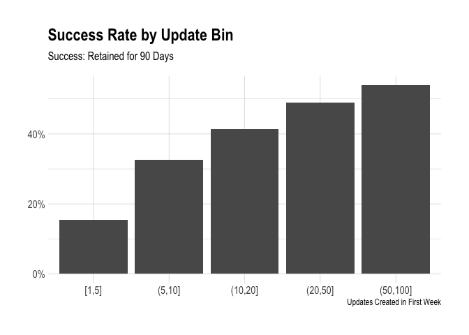
We can see that the success rate increases as the update bins increase. Over 50% of users that create 50 or more updates in their first week are retained for three months. The problem is that there are very few users that do this. We see that there is a big jump in the “success rate” from 1-5 to 6-10. Let’s zoom in there and see if there is a point with the greatest marginal return.
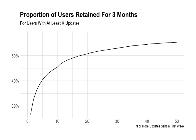
The graph below shows the proportion of users with at least X updates that were reteined for three months. We can see that there are diminishing returns, but it is tough to tell where an inflection point might be. There are certainly higher gains at the lower values os updates. One feature that is cool to see is the little bump at 11 updates. This exists because of the queue limit. Whene a user signs up for Buffer on a free plan, they can only have 10 updates scheduled at one time for a single profile.
What would this grpah look like if we zoomed into only look at 1-15 updates?
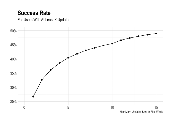
To my eyes, three or four updates seems as good a choice as any. There are clear diminishing returns after that, and a significant number of users did successfully take the action.
Profiles
We’ll take the same approach to look at profiles.
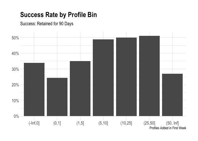
We can see that adding a single profile doesn’t quite lead to success. The biggest jump in the success rate comes between one and two profiles and five to six profiles – this is probably the case because one has to upgrade or start a trial to add that many profiles. Let’s zoom in again and try to find an inflection point in the success rates.
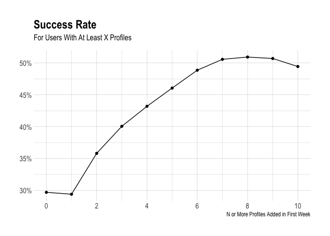
There doesn’t appear to be a clear inflection point, but we can see that the marginal increase in success is roughly linear after two profiles are added. We can’t really influence how many social accounts users have in general, so I may not recommend using profiles in an activation metric, despite the strong correlation.
Days Active
Finally we’ll look at the number of days active in the first week. How are there successful users with no days active? These users didn’t send any updates. Could they be team members? We’ll have to look into that.
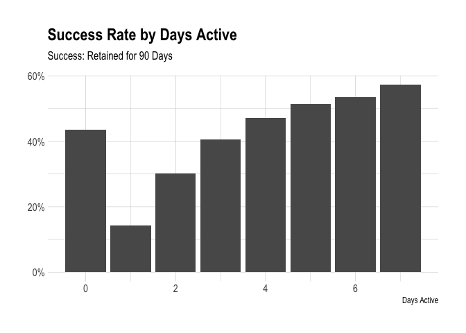
We see a significant jump in the success rate when the number of days active increases from one to two.
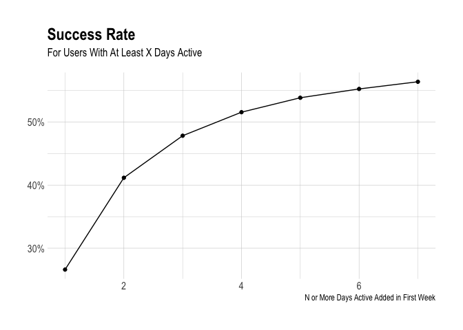
I might try a few activation metrics that include the number of days active.
Activation Metric
Let’s see what percentage of users activated if we try different combinations of activation metrics:
- At least two days active
- At least three days active
- At least two profiles
- At least three profiles
- At least three updates
- At least five updates
- At least ten updates
- At least two days active and three updates
- At least two days active and two profiles
Let’s see how the success rates would differ if we chose an activation metric of at least two days active in the first week.
# two days active
users %>%
  group_by(two_days, successful) %>%
  summarise(users = n_distinct(user_id)) %>%
  mutate(percent = users / sum(users)) %>%
  filter(successful)
## # A tibble: 2 x 4
## # Groups:   two_days [2]
##   two_days successful  users percent
##   <lgl>    <lgl>       <int>   <dbl>
## 1 F        T           94504   0.228
## 2 T        T          103457   0.412
The percent of activated users that is retained for three months is 41%, whereas the percent of non-activated users retained for three months is 23%.
What if we required the user to be active three days instead of two?
# three days active
users %>%
  group_by(three_days, successful) %>%
  summarise(users = n_distinct(user_id)) %>%
  mutate(percent = users / sum(users)) %>%
  filter(successful)
## # A tibble: 2 x 4
## # Groups:   three_days [2]
##   three_days successful  users percent
##   <lgl>      <lgl>       <int>   <dbl>
## 1 F          T          123384   0.242
## 2 T          T           74577   0.478
The proportion of users retained would increase from 24% to 48%! What if we required four days of activity?
# four days active
users %>%
  group_by(four_days, successful) %>%
  summarise(users = n_distinct(user_id)) %>%
  mutate(percent = users / sum(users)) %>%
  filter(successful)
## # A tibble: 2 x 4
## # Groups:   four_days [2]
##   four_days successful  users percent
##   <lgl>     <lgl>       <int>   <dbl>
## 1 F         T          144955   0.257
## 2 T         T           53006   0.515
The proportion of users retained would increase from 26% to 52%. That is a pretty good increase. Now let’s look at updates – what if we used the old activation metric of three updates in the first seven days?
# three updates
users %>%
  group_by(three_updates, successful) %>%
  summarise(users = n_distinct(user_id)) %>%
  mutate(percent = users / sum(users)) %>%
  filter(successful)
## # A tibble: 2 x 4
## # Groups:   three_updates [2]
##   three_updates successful  users percent
##   <lgl>         <lgl>       <int>   <dbl>
## 1 F             T           78329   0.234
## 2 T             T          119632   0.361
If we required only three updates, the proportion of users retained would increase from 23% to 36%. We might want to include a condition on the number of days active. What if we required two days active and three updates.
# see success rate
users %>%
  group_by(two_days_three_updates, successful) %>%
  summarise(users = n_distinct(user_id)) %>%
  mutate(percent = users / sum(users)) %>%
  filter(successful)
## # A tibble: 2 x 4
## # Groups:   two_days_three_updates [2]
##   two_days_three_updates successful users percent
##   <lgl>                  <lgl>      <int>   <dbl>
## 1 F                      T          97988   0.228
## 2 T                      T          99973   0.423
The percent of non-activated customers that were retained is around 23%, and the percent of activated customers that were retained is around 42%. Let’s see what would happen if we required three days active and ten updates.
# see success rate
users %>%
  group_by(three_days_ten_updates, successful) %>%
  summarise(users = n_distinct(user_id)) %>%
  mutate(percent = users / sum(users)) %>%
  filter(successful)
## # A tibble: 2 x 4
## # Groups:   three_days_ten_updates [2]
##   three_days_ten_updates successful  users percent
##   <lgl>                  <lgl>       <int>   <dbl>
## 1 F                      T          138019   0.252
## 2 T                      T           59942   0.504
The percent of users retained would increase from 25% to 50%. Nice! What if we required four days of activity?
# see success rate
users %>%
  group_by(four_days_ten_updates, successful) %>%
  summarise(users = n_distinct(user_id)) %>%
  mutate(percent = users / sum(users)) %>%
  filter(successful)
## # A tibble: 2 x 4
## # Groups:   four_days_ten_updates [2]
##   four_days_ten_updates successful  users percent
##   <lgl>                 <lgl>       <int>   <dbl>
## 1 F                     T          150529   0.261
## 2 T                     T           47432   0.527
The percent of users retained would increase from 26% to 53%. That seems like a pretty good increase!
Conclusions
Based on this data exploration, I would include the number of days active in the activation metric. Requiring four days of activity would greatly increase the likelihood of a new user being retained for three months, but only around 15% of new users reach this mark.
The greatest increase in the retention rate I saw would come when requiring at least four days active and at least 10 upates in the first week (the proportion of users retained for three months would increase from 26% to 53%). This might be a bit too hard to attain for an activation metric, so we could lower the barrier to at least three days of activity.