How Many Free Users Convert to Paying?
08 July, 2018
The question we’re going to try to answer in this analysis is “what is the percentage of new users that convert to paying within six months of signing up for Buffer?” We have to cap the amount of time users have to upgrade so that we can calculate how that rate has changed over time. Six months is an arbitrary choice, so we will also examine the percentage of new users that convert to paying within twelve months.
We will also look at the distribution of the amount of time it takes users to upgrade within each time window. Here is a quick summary of the results:
- Around 2.9% of all signups converted to paid plans at some point.
- Around 2.3% of all signups converted to a paid plan within six months of signing up.
- Around 26% of all converted users converted in the first 4 days with Buffer.
- Of the users that didn’t convert in the first four days, around 23% converted within 14 days. This means that around 77% took longer than 14 days to convert.
- Around 41% of users that didn’t convert within the first 4 days convert with 30 days. This means that, of users that don’t convert in the first 4 days, around 59% of users take more than a month to convert.
- The proportion of new users that convert to paid plans has decreased slightly from 2016 to 2017. This may be related to price changes.
- The numebr of users that convert to paid plans within 6 months has grown more slowly in 2017 than in 2016. This may also be related to price changes.
- Around 81% of users that converted to paid plans were on the Free/Individual plan for one or more days before upgrading.
- The median number of days to convert has decreased from around 14 days in 2016 to around 7 days. This may be related to trial lengths.
Data Collection and Tidying
We’ll look at all users that signed up for Buffer between January 1, 2015 and six months ago. We will also gather any subscriptions that they have created and find the first and last payments date for each.
select
  u.id as user_id
  , date(u.created_at) as signup_date
  , date(min(s.trial_start_at)) as trial_start_date
  , date(min(s.trial_end_at)) as trial_end_date
  , sum(s.successful_charges) as successful_charges
  , date(min(s.first_paid_invoice_created_at)) as first_invoice_date
  , date(max(s.last_paid_invoice_created_at)) as last_invoice_date
from dbt.users as u
left join dbt.stripe_subscriptions as s
on u.billing_stripe_customer_id = s.customer_id
and s.successful_charges >= 1
where u.created_at >= '2015-01-01'
and u.created_at < (current_date - 180)
group by 1, 2
We have 3.7 million users that have signed up between January 1, 2015 and January 6, 2018.
Exploratory analysis
We can quickly calculate the global conversion rate - i.e. how many of these 3.5 million users ended up subscribing to a paid plan at any point.
# get paid conversion rate
users %>%
  group_by(successful_charges > 0) %>%
  summarise(users = n_distinct(user_id)) %>%
  mutate(percent = users / sum(users))
## # A tibble: 2 x 3
##   `successful_charges > 0`   users percent
##   <lgl>                      <int>   <dbl>
## 1 T                         108864  0.0287
## 2 NA                       3677717  0.971
Around 108 thousand of the 3.7 million users converted to a paid plan at some point. That equates to around 2.9% of all signups.
We can also get the percentage of users that subscribed to a paid plan within six months of their signup date.
# get percentage of users that converted within 6 months
users %>%
  mutate(converted_six_months = as.numeric(first_invoice_date - signup_date) <= 180
         & !is.na(successful_charges)) %>%
  replace_na(list(converted_six_months = FALSE)) %>%
  group_by(converted_six_months) %>%
  summarise(users = n_distinct(user_id)) %>%
  mutate(percent = users / sum(users))
## # A tibble: 2 x 3
##   converted_six_months   users percent
##   <lgl>                  <int>   <dbl>
## 1 F                    3697680  0.977
## 2 T                      88901  0.0235
Around 89 thousand users converted to a paid subscription within six months of signing up for Buffer. This equates to around 2.3% of all users and 82% of all users in the sample that did eventually convert.
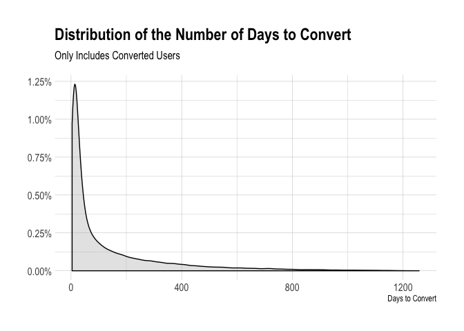
It may also be useful to visualize the distribution of the number of days it takes users to convert.

This graph shows us that most users that do convert to paid plans do so very quickly after signing up. However, there is also a very long tail of users that take a very long time to subscribe to paid plans.
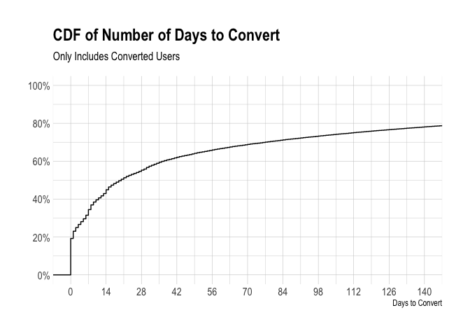
We can get a better understanding of this distribution by visualizing the cumulative distribution function (CDF).
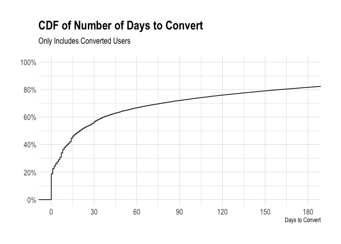
This graph is informative. Of all users in our sample that did convert, around 20% of them did so on the same day that they signed up for Buffer. This suggests that around 81% of users that ended up subscribing to a paid plan were on the free plan for more than one day.
Around 44% of users that did convert did so within 15 days of signing up, and around 57% converted within 30 days of signing up. From then onwards, the long tail of users means that a smaller and smaller percentage of users convert as the days go by.
Let’s take a look at the distribution of the number of days to convert, but this time we’ll exclude users that converted in 4 or less days. Let’s see what proportion of users this segment represents.
# get percentage of users that upgrade in more than 3 days
users %>%
  filter(!is.na(successful_charges)) %>%
  mutate(days_to_convert = as.numeric(first_invoice_date - signup_date)) %>%
  group_by(converted_in_3_days = days_to_convert <= 3) %>%
  summarise(users = n_distinct(user_id)) %>%
  mutate(percent = users / sum(users))
## # A tibble: 2 x 3
##   converted_in_3_days users percent
##   <lgl>               <int>   <dbl>
## 1 F                   80310   0.738
## 2 T                   28554   0.262
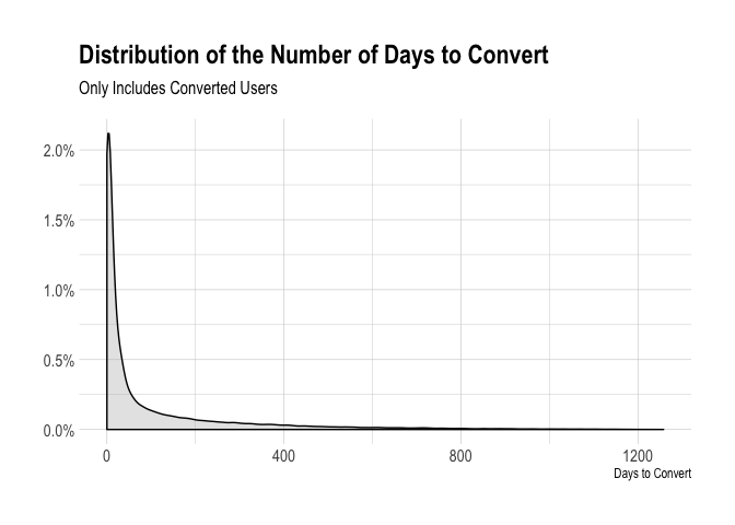
Approximately 26% of users converted within their first four days with Buffer. Now we can plot the distribution of the number of days it took to convert for users that took five or more days to convert.
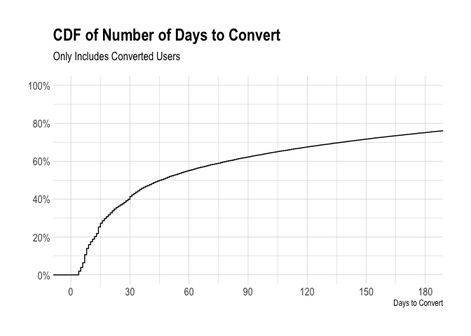
We can see that, although this distribution has a similar shape, it is different. Of the users that didn’t convert in the first four days, around 23% converted within 14 days. This means that around 77% took longer than 14 days to convert. Around 41% convert with 30 days. This means that, of users that don’t convert in the first 4 days, around 59% of users take more than a month to convert.
We see here that the long tail of the distribution is in fact very long, and contains many users.
Trials
We should note that trials mean that some users couldn’t convert for at least 7 days unless they converted early. Instead of only looking at the first paid invoice date, we can account for trials and find the minimum date between the trial start date and first invoice date. Then we could visualize that distribution with the same methods we used before.
Again we see the long tail of users that take a long time to convert. Many still convert, or start a trial that will end up converting, early on. Let’s visualize the CDF of this distribution.
Again we see that around 20% of users that converted did so on the same day in which they signed up for Buffer. Around 35% of users that converted did so within 7 days of signing up, and around 45% converted within two weeks of signing up.
Now let’s explore how the conversion rate has changed over time.
Conversion Rate Over Time
First we’ll need to group users by the week in which they signed up for Buffer.
# get signup week
users <- users %>%
  mutate(converted_six_months = as.numeric(first_invoice_date - signup_date) <= 180,
         signup_week = floor_date(signup_date, unit = "weeks")) %>%
  replace_na(list(converted_six_months = FALSE))
Now we can plot the conversion rate over time, grouping by the signup week.
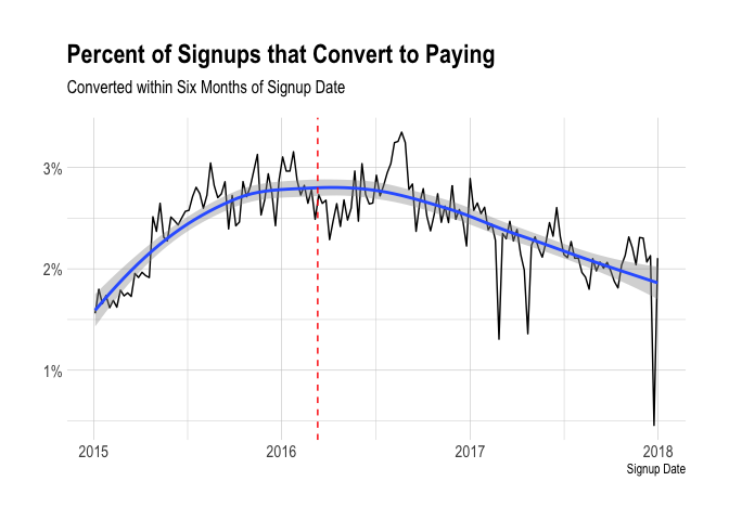
We can see that the rate at which users subscribe to paying subscriptions increased throughout 2015 and stayed roughly level around 2.75% over the course of 2016. In 2017 it seems that the rate at which users converted decreased slightly.
The dotted red line represents that date that we doubled the prices of the Business plans. This would naturally lead to a reduction in the percentage of users that subscribe to paid plans.
It may be useful to also look at the raw number of users that converted to paid plans within six months of signing up for Buffer.
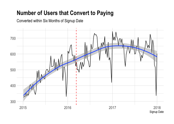
We can see here that the number of users converting to paid plans has increased steadily until the beginning of 2017. Since 2017, the number of users converting to paid plans within six months of signing up has remained roughly level.
The dotted red line represents the date that we changed the prices of the Business plans. We could expect a natural decrease in the number of users that subscribe to paid plans after that date.
Conversion Rate by Signup Source
Let’s examine the conversion rates and segment users by how they signed up for Buffer. They could have used social signin or supplied an email address and password. This data lives in the actions_taken table, so we’ll need to query it for the data we need. We’ll only look at signups from the past year.
select
  id
  , date
  , user_id
  , json_extract_path_text(extra_data, 'client_id') as client_id
  , json_extract_path_text(extra_data, 'client_name') as client_name
  , nullif(split_part(full_scope, ' ', 2), '') as signup_option
from actions_taken
where nullif(split_part(full_scope, ' ', 1), '') = 'signup'
and date > (current_date - 730)
Great, now let’s join the signups dataframe to the users dataframe.
# join signups and users
user_signups <- signups %>%
  select(user_id, client_name, signup_option) %>%
  inner_join(users, by = 'user_id')
Now we can plot the conversion rate over time for each signup option.
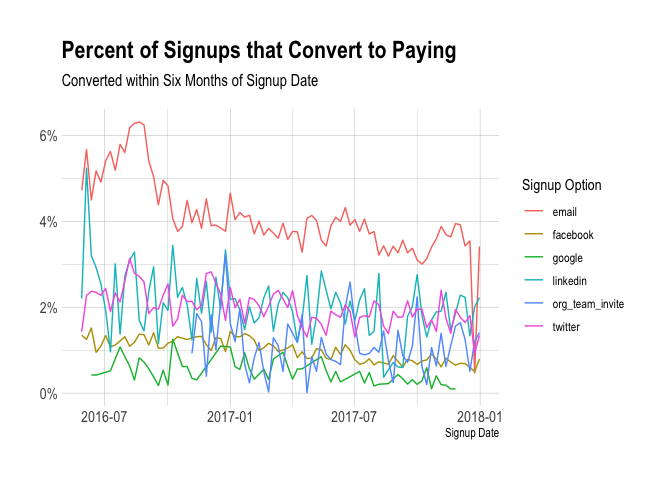
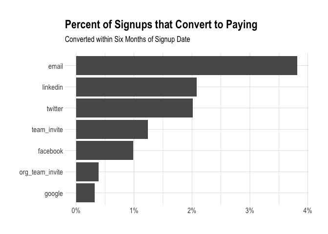
It’s difficult to compare the different networks, but it’s easy to see that users that sign up with an email address convert at the highest rate. Let’s make bar plots of the total six-month conversion rates so that we can better compare the social networks.
Now let’s compare users that signed up via web and via mobile.
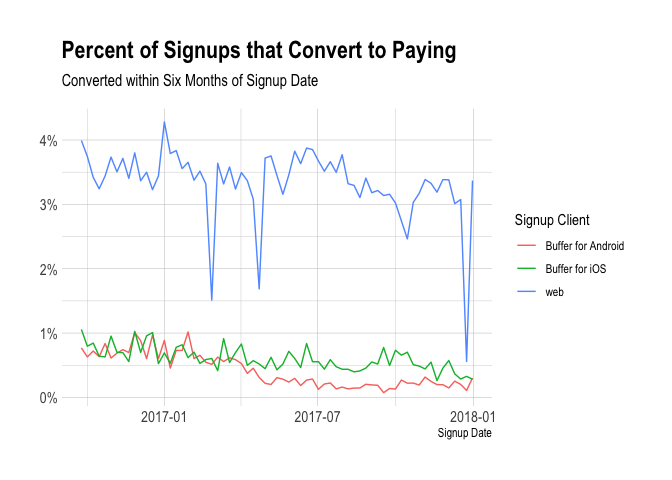
It’s interesting to see that users that signup via web convert much better! It makes sense though, since we aren’t counting mobile subscriptions here. I might discount these findings because of this fact.
Days to Convert Over Time
For each signup week, we can calculate the median number of days it took for users to convert. Then, we can plot that median value over time to get a sense of how long it’s taken users to convert historically.
# get days to convert
users %>%
  mutate(days_to_convert = as.numeric(first_invoice_date - signup_date)) %>%
  filter(converted_six_months & !is.na(successful_charges)) %>%
  group_by(signup_week) %>%
  summarise(med_days_to_convert = median(days_to_convert)) %>%
  ggplot(aes(x = signup_week, y = med_days_to_convert)) +
  geom_line() +
  geom_smooth(method = 'loess') +
  theme_ipsum() +
  labs(x = "Signup Week", y = NULL, title = "Median Number of Days to Convert",
       subtitle = "Users That Converted Within Six Months")
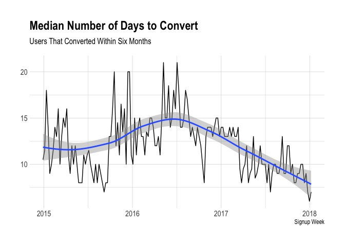
We can see that the median number of days to convert has declined slightly from around 14 days in 2016 to around 7 days in 2017.